WinNonlin Classic models include the following. Many of the WinNonlin Models can be run using the NLME engine (even if you do not have an NLME license). This is done by setting up a Phoenix Model object for individual modeling and using the Set WNL Model button to select the model. See “PK model options” in the Phoenix NLME documentation for more information. Refer to “An example of individual modeling with Phoenix model” for an illustration of how a dataset can be fitted to a two-compartment model with first-order absorption in the pharmacokinetic model library using either the WinNonlin PK Model or a Phoenix Model GUI.
-
Dissolution Models
Choose from Hill, Weibull, Double Weibull, or Makoid-Banakar dissolution models. -
Indirect Pharmacodynamic Response Models
Four basic models have been developed for characterizing indirect pharmacodynamic responses after drug administration. These models are based on the effects (inhibition or stimulation) that drugs have on the factors controlling either the input or the dissipation of drug response. See “Indirect Response models” for more details. -
Linear Models
Phoenix includes a selection of models that are linear in the parameters. See “Linear models” for more details on available models. Refer to “Linear Mixed Effects” for more sophisticated linear models. -
Michaelis-Menten Models
Phoenix’s Michaelis-Menten models are one-compartment models with intravenous or 1st order absorption, and can be used with or without a lag time to the start of absorption. For more on Phoenix’s Michaelis-Menten models, see “Michaelis-Menten models”. Information on required constants is available in “Dosing constants for the Michaelis-Menten model”. -
Pharmacodynamic Models
Phoenix includes a library of eight pharmacodynamic (PD) models. The PD models include simple and sigmoidal Emax models, and inhibitory effect models. For more on Phoenix’s PD models, see “Pharmacodynamic models”. -
Pharmacokinetic Models
Phoenix includes a library of nineteen pharmacokinetic (PK) models. The PK models are one to three compartment models with intravenous or first-order absorption, and can be used with or without a lag time to the start of absorption. For more on Phoenix’s PK models, see “Pharmacokinetic models”. See also the “PK model examples”. -
PK/PD Linked Models
When pharmacological effects are seen immediately and are directly related to the drug concentration, a pharmacodynamic model is applied to characterize the relationship between drug concentrations and effect. When the pharmacologic response takes time to develop and the observed response is not directly related to plasma concentrations of the drug a linked model is usually applied to relate the pharmacokinetics of the drug to its pharmacodynamics.
The PK/PD linked models can use any combination of Phoenix’s Pharmacokinetic models and Pharmacodynamic models. The PK model is used to predict concentrations, and these concentrations are then used as input to the PD model. This means that the PK data are not modeled, so the linked PK/PD models treat the pharmacokinetic parameters as fixed, and generate concentrations at the effect site to be used by the PD model. Model parameter information is required for the PK model in order to simulate the concentration data. Refer to “PD output parameters in a PK/PD model” for parameter details. -
User-Defined ASCII Models
Phoenix does not support the creation of ASCII models. ASCII models have been deprecated in favor of the Phoenix Modeling Language (PML). However, users can still import and run legacy WinNonlin ASCII models. For more on PML, see the PML “PML Capabilities”. Refer to “ASCII Model dosing constants” for details on required constants.
Note:There can be a loss of accuracy in WNL Classic Modeling univariate confidence intervals for small sample sizes (NDF < 5). The Univariate CIs in WNL use an approximation for the t-value which is very accurate when the degrees of freedom is at least five, but loses accuracy as the degrees of freedom approaches one. The degrees of freedom are the number of observations minus the number of parameters being estimated (not counting parameters that are within the singularity tolerance, i.e., nearly completely correlated).
In extremely rare instances, the nonlinear modeling core computational engine may get into an infinite loop during the minimization process. This infinite looping will cause Phoenix to “hang” and the application must be shutdown using the Task Manager. The process wnlpk32.exe may also need to be shutdown. The problem typically occurs when the parameter space in which the program is working within is very flat. To work around the problem, it is first suggested that the user change the minimization algorithm found on the Engine Settings tab to Nelder-Mead and retry the problem. If this fails to correct the problem, varying the initial estimates and/or using bounds on the parameters may allow processing to complete as expected.
Use one of the following to add a WinNonlin Classic Model object to a Workflow:
Right-click menu for a Workflow object: New > NCA and Toolbox > WNL6 Classic Modeling > [object name].
Main menu: Insert > NCA and Toolbox > WNL6 Classic Modeling > [object name].
Right-click menu for a worksheet: Send To > NCA and Toolbox > WNL6 Classic Modeling > [object name].
Note:To view the object in its own window, select it in the Object Browser and double-click it or press ENTER. All instructions for setting up and execution are the same whether the object is viewed in its own window or in Phoenix view.
Use the Main Mappings panel to identify how input variables are used in a model. A separate analysis is performed for each profile. Required input is highlighted orange in the interface.
•None: Data types mapped to this context are not included in any analysis or output.
•Sort: Categorical variable(s) identifying individual data profiles, such as subject ID and treatment in a crossover study. A separate analysis is done for each unique combination of sort variable values.
•X: For Dissolution, Indirect Response, Linear, PD, and PK/PD Linked Models. The independent variable in a dataset.
•Y: For Dissolution, Indirect Response, Linear, PD, and PK/PD Linked Models. The dependent variable a dataset. Not needed if the Simulation checkbox is selected.
•Time: For Michaelis-Menten, PK, and ASCII Models. Nominal or actual time collection points in a study.
•Concentration: For Michaelis-Menten, PK Models, and ASCII Models. Drug concentration values in the blood. Not needed if the Simulation checkbox is selected.
•Function: For ASCII Models. Model function.
•Carry: Data variable(s) to include in the output worksheets. Note that time-dependent data variables (those that change over the course of a profile) are not carried over to time-independent output (e.g., Final Parameters), only to time-dependent output (e.g., Summary).
•Weight: For Indirect Response, PK, PD, and PK/PD Linked Models. Used if weighting data is contained in the dataset. This column is only available if User Defined and Source are selected in the Weighting/Dosing Options tab.
Note:When using a PK operational object, external worksheets for stripping dose, units and initial estimates can be accessed in different ways. The differences will occur if there is more than 1 row of information on these external worksheets that correspond to one or more individual profiles of data of the Main input worksheet.
In such cases, the stripping dose for PK models will be determined as the first value found on that external worksheet whereas the units and initial parameters will be based on the last row found on those external worksheets (for any given profile). To avoid any confusion stemming from these differences, it is suggested that external worksheets maintain a one-to-one row-based correspondence to the Main input profiles whenever possible.
Available for Indirect Response, PK, and PK/PD Linked Models only, the Dosing panel allows users to type or map dosing data for the different models. The Dosing panel mapping columns change depending on the PK model type selected in the Model Selection tab. Required input is highlighted orange in the interface.
If multiple sort variables have been mapped in the Main Mappings panel, the Select sorts dialog is displayed so that the user can select the sort variables to include in the internal worksheet. Required input is highlighted orange in the interface.
•None: Data types mapped to this context are not included in any analysis or output.
•Sort: Sort variables.
•Time: The time of dose administration.
•Dose: The amount of drug administered. Dosing units are used.
•End Time: The end time of the infusion.
•Infusion Length: The total amount of time for an IV infusion. Only used in conjunction with a bolus dose.
•Bolus: Amount of the bolus dose.
•Amount Infused: Total amount of drug infused. Dosing units are used.
Note:If the dosing data is entered using the internal dosing worksheet, and different profiles require different numbers of doses, then leave the Time, End Time, Dose, Infusion Length, Bolus, or Amount Infused cells blank for profiles that require less than the highest number of doses.
When using an internal worksheet, click the Rebuild button to reset the worksheet to its default state and delete all entered values.
The Initial Estimates panel allows users to type or map initial values and lower and upper boundaries for different indirect response parameters.
Note:Multiple-dose datasets require users to provide initial parameter values. For more on setting initial parameter estimates, see the “Parameter Estimates and Boundaries Rules” section.
If initial estimates and parameter boundaries for ASCII models are not set in the code, then they must be set in the Initial Estimates panel.
In datasets containing multiple sort variables, the initial estimates must be provided for each level of the sort variables unless the Propagate Final Estimates checkbox is selected. Checking this box applies the same types of parameter calculations and boundaries to all sort levels. Required input is highlighted orange in the interface.
If multiple sort variables have been mapped in the Main Mappings panel, the Select sorts dialog is displayed so that the user can select the sort variables to include in the internal worksheet.
•None: Data types mapped to this context are not included in any analysis or output.
•Sort: Sort variables.
•Parameter: Model parameters such as v (volume) or km (Michaelis constant).
•Initial: Initial parameter estimate values.
•Fixed or Estimated: For Dissolution models. Whether the initial parameter is fixed or estimated.
•Lower: Lower parameter boundary.
•Upper: Upper parameter boundary.
The lower and upper values limit the range of values the parameters can take on during model fitting. This can be very valuable if the parameter values become unrealistic or the model will not converge. Although bounds are not always required, it is recommended that Lower and Upper bounds be used routinely. If they are used, every parameter must be given lower and upper bounds.
The Phoenix default bounds are zero for one bound and ten times the initial estimate for the other bound. For models with parameters that may be either positive or negative, user-defined bounds are preferred.
Note:For the WinNonlin Generated Initial Parameter Values option with Dissolution models, to avoid getting pop-up warnings that “WinNonlin will determine initial estimate” when using the Initial Estimates internal worksheet setup, delete the initial values and change the menu option from Estimated to Fixed before entering the initial estimates. Once the dropdown is changed from Fixed to Estimated, the initial value entered cannot be deleted and the warning pop-up will be displayed. Note that this situation does not affect the estimation process, as the entered initial value will not be used and WinNonlin will estimate the initial value as requested.
When using an internal worksheet, click the Rebuild button to reset the worksheet to its default state and delete all entered values.
This panel is available for Indirect Response and PK/PD Linked models only.
Note:Users are required to enter initial PK parameter values in the PK Parameters panel in order for the model to run.
To display the units in the PK Parameters panel, units must be included in the time, concentration, and dose input data and the concentration units entered in the PK Units text field in the Model Selection tab.
If multiple sort variables have been mapped in the Main Mappings panel, the Select sorts dialog is displayed so that the user can select the sort variables to include in the internal worksheet. Required input is highlighted orange in the interface.
•None: Data types mapped to this context are not included in any analysis or output.
•Sort: Sort variables.
•Parameter: Name of the parameter.
•Value: Value of the parameter.
When using an internal worksheet, click the Rebuild button to reset the worksheet to its default state and delete all entered values.
For all WNL Classic Models except Michaelis-Menten, an object’s display units can be changed to fit a user’s preferences. Required input is highlighted orange in the interface.
Depending on the type of model, there are some prerequisites for setting preferred units:
•For Indirect Response and PK Models, the Time, Concentration, and Dose data must all contain units before users can set preferred units.
•For PD and PK/PD Linked Models, the data mapped to the X and Y contexts must all contain units before users can set preferred units.
•For ASCII Models, units must be set in the ASCII model code.
Each parameter used in a model and the parameter’s default units are listed in the Units panel.
•None: Data types mapped to this context are not included in any analysis or output.
•Name: Model parameters associated with the units.
•Default: The model object’s default units.
•Preferred: The user’s preferred units for the parameter.
When using an internal worksheet, click the Rebuild button to reset the worksheet to its default state and delete all entered values.
Note:if you see an “Insufficient units” message in the table, check that units are defined for time and concentration in your input.
The Stripping Dose panel is available when one of the macro constant PK models that use a stripping dose is specified in the Model Selection tab (i.e., models 8, 13, 14, 17, or 18). This panel is used to enter the stripping dose amount, which is the dose associated with initial parameter values for macro constant models.
If a user selects a macro constant PK model and provides user-specified initial estimates, then the user must specify the associated dose. If a user chooses to have Phoenix generate initial parameter values, then the stripping dose is identical to the administered dose.
•None: Data types mapped to this context are not included in any analysis or output.
•Sort: Sort variables.
•Dose: The stripping dose.
If multiple sort values have been mapped in the Main Mapping panel, the Select sorts dialog is displayed so that the user can select the sort variables to include in the internal worksheet.
The Constants panel is available only for Michaelis-Menten and ASCII Models and allows users to type or map dosing data for the model. Specific dosing information is determined using dosing constants. For more on how constants relate to dosing in Michaelis-Menten models, see “Dosing constants for the Michaelis-Menten model”. For more on how constants relate to dosing in ASCII models, see “ASCII Model dosing constants”.
When using an external worksheet for Constants, the Number of Constants will be determined from the number of rows per profile after mapping the following:
•None: Data types mapped to this context are not included in any analysis or output.
•Sort: Sort variables.
•Order: The number of dosing constants used.
•Value: The value for each dosing constant. For example, the value for CON[0] is 1 if the model is single-dose.
For an internal worksheet, set the Number of Constants on the Options panel, or specify NCON in the model text, to expand the internal worksheet for entering the Constants.
The Format panel is only available for ASCII Models and is used to map ASCII code to an ASCII model. Users can view and edit ASCII model code in this panel.
-
Check the Use internal Text Object checkbox to edit the ASCII code.
Phoenix displays a message box asking users if they want to copy the ASCII code to an internal source:
•Click Yes to have the ASCII code copied to the internal text editor.
•Click No to remove the ASCII code and start with a blank internal text editor.
If ASCII code was previously mapped to the WNL5 ASCII Format panel then that code is displayed in the internal text editor, instead of a blank panel.
More information on the text editor is available on the Syncfusion website.
The Model Selection tab for most of the WNL Classic Models allows users to select a model and whether or not the model uses simulated data/clearance parameter. (For the ASCII Model, the Model Selection tab contains weighting options as described in the “Weighting/Dosing Options tab” description.)
-
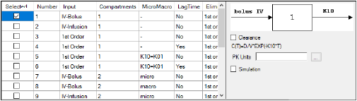
Check the checkbox beside the model number to choose it. For Dissolution models, click an option button to select a model.
Refer to any of the following sections for model details:
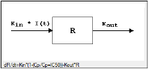
Selecting a model displays a diagram beside the model selection menu that describes the model’s functions. The model’s equation is listed beneath the diagram.
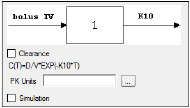
-
Set the options for the selected model.
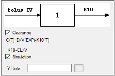
•For Indirect Response, PK, and PK/PD Linked models, select the Clearance checkbox to add a clearance parameter to the model. (The clearance parameter option is not available for PK models 8, 10, 13, 14, 17, 18, or 19.)
•For Michaelis-Menten Models, use the Number of Constants box to type or select the number of dosing constants used per profile. (For more on how the number of constants corresponds to the number, amount, and time of doses, see “Dosing constants for the Michaelis-Menten model”.)
•For PK/PD Linked Models, enter concentration units in the PK Units text field or click the Units Builder  button to use the Units Builder dialog.
Note:For PK/PD Linked Models, to view all PK parameter units in the PK Parameters panel, users must supply concentration units in the PK Units text field in the Model Selection tab and dose units in the Weighting/Dosing Options tab.
-
Check the Simulation checkbox to simulate concentration data. Enter units for the simulated data in the Y Units text field or click the Units Builder
 button to use the Units Builder dialog.
If the Simulation checkbox is selected then no concentration variable is required to run the model.
The Linked Model tab allows users to select the model to link with model specified in the Model Selection tab. It is available only for the Indirect Response and PK/PD Linked Models.
-
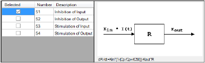
Check the checkbox beside the model number to choose it.
For more on these models, see “Indirect Response models”. For PK/PD Linked Models, see “Pharmacodynamic models”.
For a list of PD output parameters used in linked PK/PD models, see “PD output parameters in a PK/PD model”.
Selecting a model displays a diagram beside the model selection menu that describes the model’s functions. The model’s equation is listed beneath the diagram.
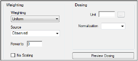
The Weighting Options tab (in Dissolution, Linear, M-M, and PD Model objects) and the Weighting/Dosing Options tab (in Indirect Response, PK, and PK/PD Linked Model objects) allows users to select a weighting scheme and specify and preview dosing options.
-
Use the Weighting menu to select one of six weighting schemes:
•User Defined: Weights are read from a column in the dataset.
•Uniform: Users can enter custom observed to or predicted to the power of N values. If selected, then users must select Observed or Predicted in the Source menu and type the power value in the Power to text field.
•1/Y: Weight the data by 1/observed Y.
•1/Yhat: Weight the data by 1/predicted Y (iterative reweighting).
•1/(Y*Y): Weight the data by 1/observed Y2.
•1/(Yhat*Yhat): Weight the data by 1/predicted Y2 (iterative reweighting).
-
Use the Source menu to select one of three weighting sources:
•Source: Selecting this option sets the weighting to User Defined and adds a Weight column to the Main Mappings panel. If selected, users must map the weighting column in the dataset to the Weight context in the Main Mappings panel.
•Observed: Select to use weighted least squares. This is the default selection for 1/Y and 1/(Y*Y). The default power for 1/Y is –1 and for 1/(Y*Y) it is –2.
•Predicted: Select to use iterative reweighting. This is the default selection for 1/Yhat and 1/(Yhat*Yhat). The default power for 1/Yhat is –1 and for 1/(Yhat*Yhat) it is –2.
-
Type a power value in the Power to text field. (This option is disabled if Source is set to Source.)
•Entering -1 automatically sets the weighting to 1/Y (if Observed is the source) or 1/Yhat (if Predicted is the source).
•Entering -2 automatically sets the weighting to 1/(Y*Y) (if Observed is the source) or 1/(Yhat*Yhat) (if Predicted is the source).
-
Check the No Scaling checkbox to not scale the weighting for observed weighting values.
When weights are contained in a dataset or Observed is selected as the source, the weights for individual data values are scaled so that the sum of weights for each function is equal to the number of data values. Weights must not be 0 (zero) in order to scale.
Scaling has no effect on the model fitting, because the weights of the observations are proportionally the same. However, scaling weights provides increased numerical stability.
Available for Indirect Response, PK, and PK/PD Linked models.
-
Enter the dosing unit in the Unit text field or click the
 button to use the Units Builder dialog to set the dosing unit.
Note:For Indirect Response Models, to view all PK parameter units in the PK Parameters panel, users must supply units for the time and concentration data in the input and specifying dose units in the Weighting/Dosing Options tab.
For PK/PD Linked Models, to view all PK parameter units in the PK Parameters panel, users must supply concentration units in the PK Units text field in the Model Selection tab and dose units in the Weighting/Dosing Options tab.
-
Use the Normalization menu to select the appropriate factor, if the dose amount is normalized by subject body weight or body mass index. Options include: None, kg, g, mg, m**2, 1.73 m**2.
Dose normalization usage:
•If doses are in milligrams per kilogram of body weight, select mg as the dosing unit and kg as the dose normalization.
•The Normalization menu affects the output parameter units. For example, if dose volume is in liters, selecting kg as the dose normalization changes the units to L/kg.
•Dose normalization affects units for all volume and clearance parameters in PK models.
-
Type the number of doses per profile into the # Doses text field. (Only enabled if an internal worksheet is used for Dosing.)
If different profiles require different numbers of doses, enter the highest number of doses. -
Click Preview Dosing to view a preview of dose option selections.
If an external dosing data worksheet is used to provide dosing data, then the preview window will show the number of doses and dosing time points per profile. Click OK to close the preview window.
All iterative estimation procedures require initial estimates of the parameter values. Phoenix computes initial estimates via curve stripping for single-dose models. For all other situations, including multiple-dose models, users must provide initial estimates or boundaries to be used by Phoenix in creating initial estimates. Parameter boundaries provide a basis for grid searching initial parameter estimates, and also limit the estimates during modeling. This is useful if the values become unrealistic or the model does not converge. For more on setting initial parameter estimates, refer to “Parameter Estimates and Boundaries Rules”.
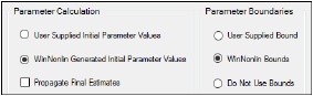
Set the parameter calculation method:
Note:The default minimization method, Gauss-Newton (Hartley) (located in the Engine Settings tab), and the Parameter Boundaries option Do Not Use Bounds are recommended for all Linear models.
-
Select the User Supplied Initial Parameter Values option button to enter initial parameter estimates in the Initial Estimates panel.
Or
Select the WinNonlin Generated Initial Parameter Values option button to have Phoenix determine the initial parameter values.
•If the User Supplied Bounds option button is selected, Phoenix uses curve stripping to provide initial estimates. If curve stripping fails, then Phoenix uses the grid search method.
•If the WinNonlin Bounds option button is selected, Phoenix uses curve stripping to provide initial estimates, and then applies boundaries to the model parameters for model fitting. If curve stripping fails, the model fails because Phoenix cannot use grid search for initial estimates without user-supplied boundaries.
-
Check the Propagate Final Estimates checkbox to propagate initial parameter estimates across all sort levels.
This option is available when more than one sort variable is used in the main dataset.
If this option is selected, then initial estimates and boundaries are entered or mapped only for the first sort level. The final parameter estimates from the first sort level provide the initial estimates for each consecutive sort level.
Set the boundary calculation method:
Parameter boundaries provide a basis for grid searching initial parameter estimates, and also limit the estimates during modeling. This is useful if the values become unrealistic or the model does not converge. For more on using parameter boundaries, refer to “Parameter Estimates and Boundaries Rules”.
-
Select the User Supplied Initial Bounds option to enter parameter boundaries in the Initial Estimates panel.
Or
Select the WinNonlin Bounds option to have Phoenix determine the parameter boundaries.
Or
Select the Do No Use Bounds option to not use parameter boundaries.
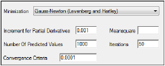
The Engine Settings tab provides control over the model fitting algorithm and related settings.
-
Use the Minimization menu to select the method to use with the Indirect Response model.
Method 1: The Nelder-Mead algorithm does not require the estimated variance-covariance matrix as part of its algorithm, so it often performs very well on ill-conditioned datasets. Ill-conditioned indicates that, for the given dataset and model, there is not enough information contained in the data to precisely estimate all of the parameters in the model or that the sum of squares surface is highly curved. Although the procedure works well, it can be slow, particularly when used to fit a system of differential equations.
Method 2: Gauss-Newton (Levenberg and Hartley) is the default algorithm and performs well on a wide class of problems, including ill-conditioned datasets. Although the Gauss-Newton method does require the estimated variance-covariance matrix of the parameters, the Levenberg modification suppresses the magnitude of the change in parameter values from iteration to iteration to a reasonable amount. This enables the method to perform well on ill-conditioned datasets.
Method 3: Gauss-Newton (Hartley) is another Gauss-Newton method. It is not as robust as Methods 1 and 2 but is extremely fast. Method 3 is recommended when speed is a consideration or when maximum likelihood estimation or linear regression analysis is to be performed. It is not recommended for fitting complex models.
Note:The use of bounds is recommended with Methods 2 and 3. For linear regressions, use Method 3 without bounds.
-
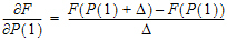
In the Increment for Partial Derivatives text field, type the incremental value that the parameter value is to be multiplied by.
Nonlinear algorithms require derivatives of the models with respect to the parameters. The program estimates these derivatives using a difference equation. For example ( =the increment with which the parameter value is multiplied)
|
|
(1) |
-
In the Number of Predicted Values text field, type the number of predicted values used to determine the number of points in the predicted data.
Use this option to create a dataset that will plot a smooth curve. When fitting or simulating multiple dose data, the predicted data plots may be much improved by increasing the number of predicted values. The minimum allowable value is 10; the maximum is 20,000.
If the number of derivatives is greater than zero (i.e., differential equations are used), this command is ignored and the number of predicted points is equal to the number of points in the dataset.
For compiled models without differential equation, the default value is 1000. The default for user models is the number of data points in the original dataset. This value may be increased only if the model has no more than one independent variable.
Note:To better reflect peaks (for IV dosing) and troughs (for extravascular, IV infusion and IV bolus dosing), the predicted data for the built-in PK models includes dosing times, in addition to the concentrations generated. For all three types, concentrations are generated at dosing times; in addition, for infusion models, data are generated for the end of infusion.
-
In the Convergence Criteria text field, type the criterion value used to determine convergence.
The default is 0.0001. Convergence is achieved when the relative change in the residual sum of squares is less than the convergence criterion. -
Leave the Meansquare text field blank, unless the mean square needs to be a fixed value in order to compute the variance in a model.
The variance is normally a function of the weighted residual SS/df, or the Mean Square. For certain types of problems, when computing the variance, the mean square needs to be set to a fixed value. -
Leave the Iterations text field set to its default value, unless the purpose of the model is to evaluate it, and not fit it.
The default iteration values are:
•500 for Nelder-Mead minimization. Each iteration is a reflection of the simplex.
•50 for Gauss-Newton (Levenberg and Hartley) or Gauss-Newton (Hartley) minimizations.
-
Type a value of 0 (zero) in the Iterations text field if the purpose of the model is evaluation.
A value of 0 requires users to supply their own initial parameter values and all output will use the initial estimates as the final parameters.
-
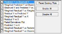
Use the checkboxes to toggle the creation of graphs.
-
Click Reset Existing Plots to clear all existing plot output.
Each plot in the Results tab is a single plot object. Every time a model is executed, each object remains the same, but the values used to create the plot are updated. This way, any styles that are applied to the plots are retained no matter how many time the model is executed.
Clicking Reset Existing Plots removes the plot objects from the Results tab, which clears any custom changes made to the plot display. -
Use the Enable All and Disable All buttons to check or clear all checkboxes for all plots in the list.
Note:This section is meant to provide guidance and references to aid in the interpretation of modeling output, and is not a replacement for a PK or statistics textbook.
After a Classic model is run, the output is displayed on the Results tab in Phoenix. The output is discussed in the following sections.
•Core Output: text version of all model settings and output, including any errors that occurred during modeling. See “Core Output File” for a full description.
•Settings: test version of all user-defined settings.
•Worksheet output: worksheets listing input data, modeling iterations and output parameters, as well as several measures of fit.
•Plot output: plots of observed and predicted data, residuals, and other quantities, depending on the model run.
Worksheet output contains summary tables of the modeling data and a summary of the information in the Core Output. The worksheets generated depend on the analysis type and model settings. They present the output in a form that can be used for reporting and further analyses and are listed on the Results tab underneath Output Data.
.
|
Worksheet |
Contents |
|
Condition Numbers |
Rank and condition number of the matrix of partial derivatives for each iteration. |
|
Correlation Matrix |
A correlation matrix for the parameters, for each sort level. |
|
Diagnostics |
Diagnostics for each function in the model and for the total: |
|
Differential Equations |
The value of the partial derivatives for each parameter at each time point for each value of the sort variables. |
|
Dosing Used |
The dosing regimen specified for the modeling. |
|
Eigenvalues |
Eigenvalues for each level of the sort variables. |
|
Final Parameters and Final Parameters Pivoted |
Parameter names, units, estimates, standard error of the estimates, CV% (values < 20% are generally considered to be very good), univariate intervals, and planar intervals for each level of the sort variables. |
|
Fitted Values |
(Dissolution models) Predicted data for each profile. |
|
Initial Estimates |
Parameter names, initial values, and lower and upper bounds for each level of the sort variables. |
|
Minimization Process |
Iteration number, weighted sum of squares, and value for each parameter, for each level of the sort variables. |
|
Parameters |
(Dissolution models) The smoothing parameter delta and absorption lag time for each profile. |
|
Partial Derivatives and Stacked Partial Derivatives |
Values of the differential equations at each time in the dataset. |
|
Predicted Data |
Time and predicted Y for multiple time points, for each sort level. |
|
Secondary Parameters and Secondary Parameters Pivoted |
Available for Michaelis-Menten, PK, PD, PK/PD Linked and ASCII models. |
|
Summary Tableb |
The sort variables, X, Y, transformed X, transformed Y, predicted Y, residual, weight, standard error of predicted Y, standardized residuals, for each sort level. |
|
Values |
(Dissolution models) Time, input rate, cumulative amount (Cumul_Amt, using the dose units) and fraction input (Cumul_Amt/test dose or, if no test doses are given, then fraction input approaches one) for each profile. |
|
Variance Covariance Matrix |
A variance-covariance matrix for the parameters, for each sort level. |
|
User Settings |
Model number, minimization method, convergence criterion, maximum number of iterations allowed, and the weighting scheme. |
|
aAIC and SBC are only meaningful during comparison of models. A smaller value is better, negative is better than positive, and a more negative value is even better. AIC is computed as: b If there are no statements to transform the data, then X and Y will equal X(obs) and Y(obs). |
Analysis produces up to eight graphs that are divided by each level of the sort variable. Plot output is listed underneath Plots in the Results tab.
-
Cumulative Rates: (Dissolution models) Cumulative drug input vs. time.
-
Fitted Curves: (Dissolution models) Observed time-concentration data vs. the predicted curve.
-
Input Rates: (Dissolution models) Rate of drug input vs. time.
-
Observed Y and Predicted Y vs X: plots the predicted curves as a function of X, with the Observed Y overlaid on the plot. Used for assessing the model fit.
-
Partial Derivatives Plot: plots the partial derivative of the model with respect to each parameter as a function of the x variable. If f(x; a, b, c) is the model as a function of x, based on parameters a, b, and c, then df(x; a, b, c)/da, df(x; a, b, c)/db, df(x; a, b, c)/dc are plotted versus x. Each derivative is evaluated at the final parameter estimates. Data taken at larger partial derivatives are more influential than those taken at smaller partial derivatives for the parameter of interest.
-
Predicted Y vs Observed Y: plots weighted Y against observed Y. Scatter should lie close to the 45 degree line.
-
Residual Y vs Predicted Y: used to assess whether error distribution is appropriately modeled throughout the range of the data.
-
Residual Y vs X: used to assess whether error distribution is appropriately modeled across the range of the X variable.
-
Weighted Predicted Y vs Observed Y: plots weighted predicted Y against observed Y. Scatter should lie close to the 45 degree line; only produced if a non-Uniform weighting scheme is used.
-
Weighted Residual Y vs Observed Y: used to assess whether error distribution is appropriately modeled across the range of the observed Y variable; only produced if a non-Uniform weighting scheme is used.
-
Weighted Residual Y vs Predicted Y: used to assess whether error distribution is appropriately modeled across the range of the predicted variable; only produced if a non-Uniform weighting scheme is used.
-
Weighted Residual Y vs Weighted Predicted Y: used to assess whether error distribution is appropriately modeled throughout the range of the data; only produced if a non-Uniform weighting scheme is used.
-
Weighted Residual Y vs X: used to assess whether error distribution is appropriately modeled across the range of the X variable; only produced if a non-Uniform weighting scheme is used.
Users can double-click any plot in the Results tab to edit it. (See the “Plot Options tab” description for editing options.)
