The Phoenix Model Object

Structure tab

The Structure tab is used to set up the Phoenix model. When selections are made in this tab, the PML that defines the model changes. The changes to the PML can be viewed in the Model Text tab.

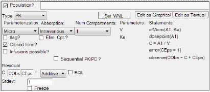
Structure model options tab set up for a PK intravenous population model

In the Type menu, select the type of Phoenix model:

•PK: See “PK model options” for PK model options.

•Emax: See “Emax model options” for Emax model options.

•PK/Emax: The options for the PK/Emax model are the same as those listed under “PK model options” and “Emax model options”.

•PK/Indirect: See “PK/Indirect model options” for Indirect model options. The options for the PK portion of the model are the same as those listed under “PK model options”

•Linear: See “Linear model options” for Linear model options.

•PK/Linear: The options for the PK/Linear model are the same as those listed under “PK model options” and “Linear model options”.

Caution:Changing the structural model after random effects have been set up can result in reordering of the random effects and changes in associated initial estimates. Caution is advised in double-checking the random effects entries after a model is changed.

Structure tab options change depending on the type of model selected.

PK model options

In the Parameterization menu, select the type of parameterization to use in the model. Each parameterization option changes the parameters and statements listed in the Structural tab.

•Micro: Model is expressed as differential equations having mass transfer rate constants associated with a compartmental model. Adds the mass transfer rate parameters, such as Ke, the rate of elimination, and writes the derivatives in terms of compartmental masses.

•Clearance: Model is expressed as differential equations having clearances associated with a compartmental model. Adds the inter-compartmental clearance parameters, such as Cl, the clearance rate. If Clearance is selected, the Saturating checkbox becomes available. Check the Saturating checkbox to convert the model to a saturable elimination model. A saturable model uses two parameters:
Km: Concentration to achieve half of maximal metabolic rate.
Vmax: The maximum metabolic rate.

•Macro: Model is expressed as a closed-form sum of exponentials. This option directly models concentration in the central compartment. Volume is not in the model but can be derived as a secondary parameter. This is the same parameterization as the WNL5 Classic model. Primary parameters are the sum of exponential terms that model concentration in the central compartment. The user can enter the dose (A1) as well as a stripping dose (A1Strip). If no stripping dose is mapped on the Main or Dosing panels, the stripping dose is assume to be equal to the dose.

•Macro1: Model is expressed as a closed-form sum of exponentials. This option models the amount in the central compartment (A) and Volume is a primary parameter. Primary parameters are the sum of exponential terms plus the parameter Volume. The amount in the central compartment is modeled as a sum of exponentials and then the Volume parameter is used to convert that amount to a concentration. Note that, because both macro options are closed-form models, the Closed form? option is removed.

Turn on the tlag checkbox to add a time delay parameter to the model.

Adding a time lag assumes that there is a fixed amount of time between drug delivery (dose time) and when the drug is introduced into the blood.
Turn on the Elim. Cpt. checkbox if urine is being analyzed or data is available for any type of elimination compartment.

Selecting this option adds a differential equation for A0, the amount of a drug excreted from the body. An elimination compartment is added to the model and included in the model code as a urinecpt statement. Basically, the urinecpt statement is like the deriv statement, except in a steady-state dosing situation, where urinecpt is ignored.

Note:Adding an elimination compartment to a Clearance model removes the Closed form? option and adds the Fe.? option for toggling the inclusion of the fraction excreted parameter.

Check the Closed form? checkbox to convert the model from a differential equation model to a closed-form algebraic model.

The closed-form model runs faster, but has some disadvantages:

•There can only be one observed variable, such as central compartment amount or concentration.

•The differential system being converted must be linear (no nonlinear kinetics).

•Any covariates used in the model must be constant for the duration of the observations. For example, no change in subject's weight as samples are collected.

Check the Infusions possible? checkbox if the model uses a constant rate of drug delivery.

Infusions can be selected for intravenous and extravascular input. Selecting this option adds an extra context for the rate of drug delivery to the Main Mappings panel. For intravenous absorption the new mapping context is A1 Rate. For extravascular absorption, the mapping context is Aa Rate. A Duration? checkbox is also added in the Structure tab. Checking this box causes the context A1 or Aa Rate to change to A1 or Aa Duration.
In the Absorption menu select the method of drug delivery.

•Intravenous: The drug is introduced directly into the blood.

•Extravascular: The drug is introduced indirectly into the blood.

Selecting the Extravascular option adds an extra parameter, Ka, which is the rate of absorption and adds an extra checkbox that allows users to set the rate of absorption equal to the rate of elimination.

Check the Ka = Ke checkbox to set the absorption rate equal to the elimination rate (the Ke parameter is removed from the model).
In the Num Compartments menu, select the number of compartments.

The default is one central compartment, and up to two peripheral compartments can be added.For each peripheral compartment added, two parameters are added to the model to account for the flow between the compartments. If macro parameterization is selected, the Num Compartments menu changes to the Num Terms menu.
In the Num Terms menu, select the number of exponential terms to use in the model.

The following table lists the parameters that are added to the model for each extra compartment or term that is selected.

	Parameterization
Number of compartments or terms	Micro	Clearance	Macro	Macro1
1	V, Ke	V, Cl	A, Alpha	V, Alpha
2	K12, K21	V2, Cl2	B, Beta	B, Beta
3	K13, K31	V3, Cl3	C, Gamma	C, Gamma

Select the Sequential PK/PD? checkbox if the PK model is part of a PK/PD model that is being fitted sequentially. This will freeze the PK portion of the model and turn its random effects into covariates. See “Sequential PK/PD Population Model Fitting” for more information.
In the Residual Error fields, define the equation used to determine the error model.

C in the residual error model represents the central compartment. Changes made in the Residual Error field are shown in the observe statement.
In the first field, type the name of the observed quantity variable or use the default (CObs).
In the second field, type the name of the epsilon variable or use the default name (CEps).

The epsilon variable represents a normal error with standard deviation as specified in the Stdev field.
In the error model type menu, select the type of error model.

The Additive error model assumes error magnitudes are constant, regardless of concentration. The error bars in the residual plots are set to Ceps. The Multiplicative error model assumes error magnitudes are proportional to concentration. The error bars are scaled by C*Ceps. The Power error model assumes the error magnitudes are proportional to the square root of concentration and the error bars are scaled by sqrtC*Ceps. See “Additional details on error models” for more information.

•If Add+Mult is selected, type a name for the parameter in the Mult Stdev field or accept the default name.

•If Mix Ratio is selected, type a name for the mixed ratio parameter in the mix Ratio field or accept the default name.

•If Power is selected, type a value for the exponent in the Power field.

•If Custom is selected, type a custom error model definition in the Defn field.

For PK models, Multiplicative followed by Power are the preferred error models over Additive. This is because PK model types usually have concentrations spanning several orders of magnitude and, on a log scale, Additive has large errors at low concentrations.

For PD model types, with effect ranges usually less than an order of magnitude, Additive is the first choice.

In the Stdev field, type a value for the standard deviation or accept the default.

The residual error cannot be less than 0.001 for all engines except Naive Pooled and QRPEM.
Select the BQL? checkbox if the dataset contains BQL values for the observation data.

A resulting worksheet of a BQL object with a censored column CObsBQL can be used as the input for a Phoenix Model with the option BQL?. If BQL? is selected, a column can be mapped to the CObsBQL context in the Main Mappings panel. This column can contain two categories of values: non-zero (censored) or zero (non-censored). If a concentration value is marked as censored (CObsBQL<>0), it means that the true value of the observation is unknown but it is not greater than the observed value (e.g., LLOQ) and then the cumulative distribution function for the normally distributed error is used to calculate the likelihood. If a concentration value is flagged as non-censored, then the probability density function is used to calculate the likelihood.

The context name CObsBQL changes based on what is typed in the observed quantity variable field. For example, instead of CObsBQL it could be ConcBQL.

Note:Phoenix models with censored data (BQL? option) use the log of the probabilities between 0 and the censored number in the log likelihoods. If the censoring numbers are very small, the loglikelihood might overflow, resulting in a Fortran error. This seems to be more often the case when using multiplicative error models. If the error occurs, try increasing the BQL value if possible or change error types.

Turn on the Use Static LLOQ? checkbox to enter a numeric value of LLOQ (>0).

In the event that CObsBQL is not mapped to a column in the dataset, then the static value of LLOQ will be used, so any observed value less than or equal to that LLOQ value is treated as censored. Only turn on the Use Static LLOQ? box to specify a static LLOQ value. However, even if a value is specified, if the CObsBQL column (or other column with a BQL flag) is mapped, the value in the observation column will be used as the LLOQ and will override the static LLOQ.
Check the Freeze checkbox to freeze the standard deviation to the value shown in the Stdev field and prevent estimation of this part of the model.
Click Set WNL Model to run Phoenix WinNonlin class model structures using Phoenix NLME.

•In the first unlabeled menu, select one of the 19 PK models, or one of the four Michaelis-Menten models, or one of the 19 PK/PD simultaneous link models. The PK/PD simultaneous link models are labeled 401 to 419 and link PK models 1 through 19 with PD model 105 (e.g., PK/PD model 407 is a linked model of PK model 7 with PD model 105). For more on PK/PD simultaneous link models, see “Differential equations in NLME”.

•If the model specified in the first unlabeled menu is not a macro-parameterization model, the CL/V checkbox is made available. Check this box to add clearance and volume parameters to the model.

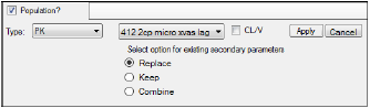
WNL model setup with additional parameters option

•If a linked model is specified in the first unlabeled menu, a second unlabeled menu is made available. Select one of eight PD models, or one of four Indirect Response models to link.

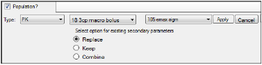
WNL linked model setup

•Each WNL model has a set of secondary parameters that available for loading when that model is selected. Use the radio buttons to indicate what should be done with secondary parameters that are already defined in the interface when the model is loaded. Choose to Replace currently defined parameters with those and load the ones from the model, Keep currently defined parameters and ignore those from the selected model, or Combine them by keeping the existing parameters and adding those from the selected model to the list.

•Click Apply to apply the selected model or models or click Cancel to exit the model selection menus without applying any changes.

Additional details on error models

The Log-additive option corresponds to a form like C*exp(epsilon). If the Log-additive error model is specified, and if there is only one error model, such as one observe statement, then the predictions and observations are log-transformed and are fit in that space. This is because the error model becomes additive in log-space, which allows for higher performance and accuracy. This affects all the plots results and residuals, because they are in log-space. The simulation tables are transformed back so they are not in log-space.

Because the logs of zero or negative numbers are not allowed, they are truncated to a value which is ¼ (0.25) of the smallest positive observation value. If the model is Log-additive, but the conditions have not been met for log-transforming to take place, the model behaves the same as Multiplicative.

The residual model that is displayed in the model text is:

observe(CObs=C*exp(CEps))

observe(CObs=exp(log(C)+CEps))

(1)

The engines implement the model by log-transforming both sides and see if the derivative of the right-hand side with respect to CEps is 1. If so, and if there is only one observe statement, then it does log-transformation.

observe(log(CObs)=log(C)+CEps)

(2)

This check is accomplished by examining the text of the model, so it can be applied to models other than built-in models.

The main advantages of Log-additive are that the engines, particularly the Lindstrom-Bates FOCE engine, can run faster when a simple additive error model is used, and the FOCE approximation can be more accurate.

Since the modeling engines in NLME can only handle a single error variable (or epsilon), and some error models are best specified as having an additive component and a multiplicative component, some complexities are needed. The Mix Ratio uses the following formula:

C+eps*(1+C*mixRatio)

(3)

where mixRatio is a fixed effect and is understood to be the multiplicative sigma divided by additive sigma.

Another way to specify a mixed error model having a fixed effect, but with the fixed effect signifying the multiplicative sigma, rather than the ratio of multiplicative to additive sigma is Add+Multi. It makes use of a built-in function called “sigma()” that can only be used in this context, and its value is the current estimate of the standard deviation of eps. The formula is:

C+eps*sqrt(1+(C*multStdev/sigma())^2)

(4)

where multStdev is the multiplicative sigma.

So when this error model is used, the additive sigma is called stdev, and the multiplicative sigma is called multStdev. Since multStdev is a fixed effect, its name can be changed as desire.

To justify the above formula, look at the variance. Suppose the additive standard deviation is called sigma1, the multiplicative standard deviation is called sigma2, and suppose the corresponding epsilons eps1 and eps2 are drawn from a unit normal distribution. Then the formula would be:

C+eps1*sigma1+C*eps2*sigma2

(5)

The variance of this is the sum of the variances from each term, or:

sigma1^2+(C*sigma2)^2

(6)

Now let r be the ratio: r=sigma2/sigma1, then the variance is:

sigma1^2+(C*r*sigma1)^2

sigma1^2 *(1+(C*r)^2)

(7)

which is the variance of:

C+eps*sqrt(1+(C*r)^2)

(8)

Then replace r with sigma2/sigma1 to obtain:

C+eps*sqrt(1+(C*sigma2/sigma1)^2)

(9)

where sigma1 is represented by the sigma() function, and sigma2 is represented by multStdev.

So, by choosing the option Add+Mult, this formula will be used to estimate both stdev (the additive standard deviation) and multStdev (the multiplicative standard deviation).

Emax model options

Check the Baseline checkbox if the model has a baseline response.
A new parameter, E0, is added to the baseline response and the Fractional checkbox is made available.
Check the Fractional checkbox if the Emax model is fractional.
Selecting this option modifies the E0 equation statement.
Check the Inhibitory checkbox if the Emax model is inhibitory.
The structural parameters EC50 and Emax change to IC50 (concentration producing 50% of maximal inhibition) and E0 (baseline effect).
Check the Sigmoid checkbox if the Emax model is sigmoidal.
A shape parameter, Gam, is added.
In the Residual Error field, define the equation used to determine the error model.

•E in the residual error model represents the effect observation.

•Changes made in the Residual Error field are shown in the observe statement.

In the first field, type the name of the observed effect variable or accept the default name of EObs.
In the second field, type the name of the epsilon variable or accept the default name of EEps.
In the error model type menu, select the type of error model. Refer to “Additional details on error models” in the PK model section for more information.
Check the BQL? checkbox if the dataset contains BQL values for the observation data.

If BQL? is selected, a column can be mapped to the EObsBQL context in the Main Mappings panel. This column can contain two values: one (censored) or zero (non-censored). If a concentration value is marked as censored, then the cumulative distribution function for the normally distributed error is used to calculate the likelihood. If a concentration value is flagged as non-censored, then the probability density function is used to calculate the likelihood.

The context name EObsBQL changes based on what is typed in the observed effect variable field. For example, instead of EObsBQL it could be EffectBQL.

In the Stdev field, type a value for the standard deviation.
Check the Freeze checkbox to freeze the standard deviation to the value shown in the Stdev field.

PK/PD Link Models can be specified by selecting a PK/Emax, PK/Indirect, or a PK/Linear model from the Type menu or by setting a PK/PD link model as discussed above.

When a PK/Emax, PK/Indirect, or a PK/Linear model is selected, there are two observation columns displayed in the mappings panel: one for concentration observations; and one for effect observations.
Check the Freeze PK? checkbox to freeze the PK parameters by removing the PK observation from the model. Only the parameters for the PD model are estimated.
Check the Sequential PK/PD? checkbox to estimate the PK and PD parameters sequentially.

Checking the Sequential PK/PD? checkbox freezes the PK portion of the model and turns its random effects into covariates to be imported from the first model, so that plasma concentration will be predicted identically to what it was predicted as in the first model. It also removes the PK observation from the model, since the PK portion of the model is not being fit. See “Sequential PK/PD Population Model Fitting” for more information.

To include a hysteresis plot, on the Run Options tab, add a Table with Times and Variables C, E, CObs, EObs, Ce for built-in models (or use the specified Variable names from graphical or textual models), and then create the desired plot from the Table output.”

PK/Indirect model options

The following options are for the Indirect portion of the PK/Indirect model. Options for the PK portion of the model are the same as those listed under “PK model options”.

In the Indirect menu, select the indirect model type:

•Stim. Limited (limited stimulation of input)

•Stim. Infinite (infinite stimulation of input)

•Inhib. Limited (limited inhibition of input)

•Inhib. Inverse (inverse inhibition of input)

•Stim. Linear (linear stimulation of input)

•Stim. Log Linear (logarithmic and linear stimulation of input)

Use the Indirect menu options to select a model in which the response formation (build-up) or degradation (loss) is stimulated or inhibited by increased concentrations. The default response setting is the build-up of the response, or the production of the response.

Click Buildup to change the response setting to a Loss, or fractional turnover rate, of response.

This constructs a model where the degradation of response is concentration dependent. For example, Loss statement with limited stimulation: deriv(E=Kin – Kout*(1+Emax*C/(C+EC50))*E)
Click Loss to change the response setting back to Buildup of the response.

This constructs a model where the formation of response is concentration dependent. For example, Buildup statement with limited stimulation: deriv(E=Kin*(1+Emax*C/(C+EC50)) – Kout*E)
Click no Exponent/Exponent to toggle between adding and removing an exponent to/from the effect statement.
The exponent parameter is gam.
The Residual Error model options for the PK model and the Indirect model are the same as the PK model options and Emax model options.

Linear model options

In the Linear menu, select the linear model type:

•E = Alpha, a constant model, where y(x)=constant.

•E = Alpha + Beta * C, a linear model, where y(x)=intercept+slope*x.

•E = Alpha + Beta * C + Gamma * C^2, a quadratic model, where y(x)=A0+A1*x+A2*x^2.

In the above equations, y is the dependent variable and x is the independent variable.

The Residual Error model options for the Linear model are the same as those for the Emax model options.