Example - Analysis of three profiles using NCA

NCA examples

This section presents several examples of the NCA operational object usage within Phoenix. Knowledge of how to do basic tasks using the Phoenix interface, such as creating a project and importing data, is assumed.

The examples include:

Analysis of three profiles using NCA
Exclusion and partial area NCA example
Sparse sampling NCA example
Urine study NCA example
Drug effect NCA example
Multiple profile analysis using NCA

Analysis of three profiles using NCA

Suppose a researcher has obtained time and concentration data following oral administration of a test compound to three subjects, and wants to perform noncompartmental analysis and summarize the results.

The completed project (NCA.phxproj) is available for reference in …\Examples\WinNonlin.

Set up the project and data for the three profiles

Create a new project named NCA.
Import the file …\Examples\WinNonlin\Supporting files\Bguide1 single dose and steady state.dat.

Note:Units must be added to the time and concentration columns before the dataset can be used in a noncompartmental analysis.

With Bguide1 single dose and steady state selected in the Data folder, go to the Columns tab (lower part of the Phoenix window) and select the Time column header in the Columns box.
Clear the Unit field and type hr.
Select the Conc column header in the Columns box.
Clear the Unit field and type ng/mL.
Or
Click the Units Builder button and use the Units Builder dialog tools

Note:Units added to ASCII datasets can be preserved if the datasets are saved in .dat or .csv file format. Phoenix adds the units to a row below the column headers. To import a .dat or .csv file with units, select the Has units row option in the File Import Wizard dialog.

Set up the NCA object for analysis of the three profiles

Noncompartmental analysis for extravascular dosing is available as Model 200 in the Phoenix model library. Phoenix displays the model type (Plasma, Urine, or Drug Effect) in the Options tab of an NCA object.

Note:The exact model used is determined by the dose type. Extravascular Input uses Model 200, IV-Bolus Input uses Model 201, and Constant Infusion uses Model 202.

Select Workflow in the Object Browser and then select Insert > NonCompartmental Analysis > NCA.
Drag the Bguide1 single dose and steady state worksheet from the Data folder to the NCA object’s Main Mappings panel.
Map the data types as follows:
Day to the Sort context (make sure to map Day first)
Subject to the Sort context
Time mapped to the Time context
Conc to the Concentration context

Prepare the dosing information from the profiles

Select Dosing in the NCA object's Setup list.
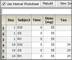
In the Dosing panel, select the Use Internal Worksheet checkbox.
Click OK in the Select sorts dialog to accept the default sort variables.
For each row:
In the Time column, enter 0.
In the Dose column, enter 55.
In the Tau column, enter 24 for the three Day 14 rows (rows 4, 5, and 6).

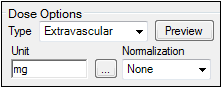
In the Dose Options area of the Options tab, type mg in the Unit field and press the Enter key.
The units are immediately added to the column header.
Extravascular is selected by default in the Type menu. Do not change this setting.

Set up the terminal elimination phase for the analysis

Phoenix attempts to estimate the rate constant Lambda Z, associated with the terminal elimination phase. Although Phoenix is capable of selecting the times to be used in the estimation of Lambda Z, this example provides Phoenix with the time range.

Specify the times to be included.

Select Slopes in the Setup list.
For each row:
In the Start Time column, type 8.
In the End Time column, type 24.
Do not type any values into the Exclusions column.
Select Slopes Selector in the Setup list.

The Time Range is selected in the Lambda Z Calculation Method menu. The Start and End times have been specified for each subject. A line is displayed on each graph that shows the Lambda Z time range.

In this example, no points are excluded from the specified Lambda Z time range. The example “Exclusion and partial area NCA example” demonstrates Lambda Z exclusions.

Specify therapeutic response options

The next step is to define a target concentration range to enable calculation of the time and area located above, below, and within that range.

Note:See “Exclusion and partial area NCA example” for an NCA example that includes computation of partial areas under the curve.

Select Therapeutic Response in the Setup list.
Select the Use Internal Worksheet checkbox.
Click OK in the sorts dialog to accept the default sort variables.
For each row:
Type 2 in the Lower column.
Type 4 in the Upper column.

Set preferred units for the analysis

The next step in setting options is to specify preferred output units. The independent variable, dependent variable, and dosing regimen must have units before preferred output units can be set.

Select Units in the Setup list.

The Units worksheet lists both the Default units and the Preferred units for each parameter. The new preferred volume unit needs to be set to L (liter).
Select the cell in the Preferred column for Volume (Vz, Vz/F, Vss).
Type L and press ENTER.

Specify NCA model options for the analysis

Four methods are available for computing the area under the curve. The default method is the linear trapezoidal rule with linear interpolation. This example uses the Linear Log Trapezoidal method: linear trapezoidal rule up to Tmax, and log trapezoidal rule for the remainder of the curve.

Use the Options tab to specify settings for the NCA model options. The Options tab is located underneath the Setup tab.

Select Linear Log Trapezoidal in the Calculation Method menu.
In the Titles field type Example of Noncompartmental Analysis.

Set an acceptance criteria rule

Acceptance criteria for Lambda Z, which are applicable to both the Best Fit method and the Time Range method, can be specified on the Rules tab. These rules are used to flag profiles where the Lambda_z final parameter does not meet the specified acceptance criteria.

Select the Rules tab.
In the Rsq_adjusted field, type 0.97 to flag any profile with an Rsq_adjusted value greater than or equal to this value.

Profiles that break the rule are flagged in the output and can be quickly filtered out of the results. The process will be illustrated later in this example.

Execute and view the results of the analysis

At this point, all of the necessary commands have been specified.

Click (Execute icon) to execute the object.
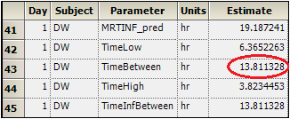
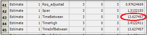
In the Results tab, select Final Parameters in the list.

Subject DW’s concentrations were within the theoretical therapeutic range for just over 13.8 hours, as reflected in the parameter TimeBetween.

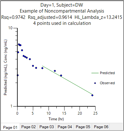
In the Results tab, select Observed Y and Predicted Y vs X in the list.

The NCA object’s plot output includes Observed Y and Predicted Y vs X graphs for each subject (switch between the plots using the tabs below the graph).

In the Results tab, select Core output in the list.

The NCA object’s Core Output text file contains user settings, a brief summary table, and final parameters output for each subject.

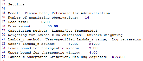
Settings portion of the Core Output

Filter out flagged profiles

In the Results tab, select Final Parameters Pivoted in the list.

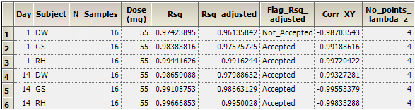
Part of the Final Parameters Pivoted worksheet

For this example, a rule was set for the value of Rsq_adjusted (see “Set an acceptance criteria rule”). The output indicates that the profile for DW broke this rule with a value of ‘Accepted’ in the Flag_Rsq_adjusted column.

To remove any profiles failing to meet acceptance criteria from the output, the Final Parameters Pivoted worksheet can be processed by the Data Wizard to delete these profiles. The worksheet is filtered on the flag values of 'Not Accepted' and identified rows are then excluded.

Note:The NCA.phxproj file does not include processing by the Data Wizard, but the information is included here as a reference.
a) Insert a Data Wizard object.
b) In the Options tab, set Action to Filter and click Add.
c) Click the Select Source icon in the Mappings panel and select the NCA Final Parameter Pivoted worksheet.
d) In the Options tab, click the Add button to the right of the Specify Filter field.
e) In the Filter Specification dialog, define the filter to Exclude rows that have a value of Not Accepted in the Flag_Rsq_adjusted column (or other “Flag_” column on which you want to filter profiles).
Once the filter is defined, execute the Data Wizard object.

Summarize the analysis output with statistics

At this point, it is convenient to summarize the results of the noncompartmental analysis using a Descriptive Statistics object. This example summarizes parameter estimates across subjects.

Select Workflow in the Object Browser and then select Insert > Computation Tools > Descriptive Statistics.
In the Descriptive Statistic’s Main Mappings panel click the Select Source icon.
Under the NCA node, select the Final Parameters worksheet and click OK.
In the Main Mappings panel, map the data types to the following contexts:
Map Day to the Sort context (make sure to map Day first).
Leave Subject mapped to None.
Map Parameter to the Sort context.
Leave Units mapped to None.
Map Estimate to the Summary context.

Note:Mapping Day and Parameter to Sort computes statistics on the parameter estimates for each day and mapping Estimate to Summary computes one statistic per parameter per day.

In the Options tab, check the Confidence Intervals and Number of SD Statistics checkboxes, but do not change the default values for these two items.
Execute the object.

The three subjects spent an average of 13.6 hours within the therapeutic concentration range on Day 1, as shown by the parameter TimeBetween.

Use ratios to compare data

The Ratios and Differences object can be used to quickly setup ratios and/or differences between parameter values in order to compare data. A description of the object can be found in “Ratios and Differences”.

In the Object Browser, click the NCA object.
In the Results list, right-click Final Parameters Pivoted and select Send To > Computation Tools > Ratios and Differences.
In the Main Mappings panel of the Ratios and Differences object, map the data types to the following contexts:
Map Day to the Filter context.
Map Subject to the Sort context.
Map the rest of the data types to the Carry context by first mapping N_Samples to Carry and then drag the corner of the selected cell all the way to the bottom of the grid. It may take a few seconds.
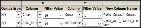
In the Options tab, set up two ratios as shown in the following image. Use the Add button to add the second row of options to the table.

Execute the object.
In the Results tab, select Ratios Differences and compare the ratios for each subject.

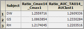
This concludes the multiple profile example.