Example - Exclusion and partial area NCA

Exclusion and partial area NCA example

This example demonstrates the exclusion of points in the terminal elimination phase and computation of partial area under the curve in the Phoenix NCA object. The time-concentration data is for a single subject and the data is provided in NCA2.csv, which is located in the Phoenix examples directory.

Noncompartmental analysis for extravascular dosing is available as model 200 in Phoenix’s noncompartmental analysis object. Phoenix always displays the model type in the NCA object’s Options tab.

Note:The exact model used is determined by the dose type. Extravascular Input uses Model 200, IV-Bolus Input uses Model 201, and Constant Infusion uses Model 202.

The completed project (NCA_PartialAreas.phxproj) is available for reference in …\Examples\WinNonlin.

Set up the NCA object

Create a project called NCA_PartialAreas.
Import the file …\Examples\WinNonlin\Supporting files\NCA2.csv.
In the File Import Wizard dialog, make select the Has units row option.
Click Finish.
Select Workflow in the Object Browser and then select Insert > NonCompartmental Analysis > NCA.
Drag the NCA2 worksheet from the Data folder to the NCA object’s Main Mappings panel to map it as the input source.
Leave Time mapped to the Time context.
Map Conc to the Concentration context.

Prepare the dosing information

In this example, one dose of 70 mg was administered at time zero.

Select Dosing in the Setup list.
In the Dosing panel, check the Use Internal Worksheet checkbox.
In the first cell in the Time column type 0.
In the first cell in the Dose column type 70.
Do not enter any values in the Tau column.
Extravascular is selected by default in the Type menu in the Options tab. Do not change this setting.
In the Unit field type mg and press the Enter key.

Set up the terminal elimination phase

Phoenix attempts to estimate the rate constant Lambda Z associated with the terminal elimination phase. Although Phoenix is capable of selecting the times to be used in the estimation of Lambda Z, this example provides Phoenix with the time range.

Select Slopes in the Setup list.
In the Slopes panel, type 0.33 in the Start Time column.
Type 2.5 in the End Time column.
Exclude the data point at 1.5 by typing 1.5 in the Exclusions column and press the Enter key.
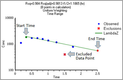
Select Slopes Selector in the Setup list.

The Start and End times and the Exclusion are marked on the graph display.

Specify the AUCs to calculate

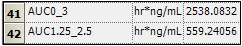
Partial areas under the curve are computed for zero to 3.0 hours and 1.25 to 2.5 hours.

Select Partial Areas in the Setup list.
Select the Use Internal Worksheet checkbox.
In the Options tab, change the Max # of Partial Areas pull-down menu to 2.
In the first row, type 0 in the Start Time column and type 3 in the End Time column.
In the second row, type 1.25 in the Start Time column, type 2.5 in the End Time column and press the Enter key.

Specify the NCA model options

This example includes titles in the graph output and uses the Linear Log Trapezoidal method to calculate areas under the curve.

Use the Options tab to specify settings for the NCA model options.

The default setting for Model Type is Plasma (200-202). Do not change this setting.

Note:The exact model type (200, 201, or 202) is determined by the dose type.

Select Linear Log Trapezoidal in the Calculation Method menu.
In the Titles field type A Second NCA Example.

Request a concentration at a specified time

Set up a request to calculate the concentration at time 0.25 and include the information in the results.

Select the User Defined Parameters tab.
Check the Include with Final Parameters check box.
In the Compute Concentrations at Times field, enter 0.25.

Define a new parameter

Add a new dose-normalized parameter.

In the User Defined Parameters tab, click the Add button.
Enter AUCall_D in the Parameter column.
Enter AUCall/Dose in the Definition column.
Enter hr*ng/mL/mg in the Units Label column.

Execute and view the NCA results

All necessary settings are complete.

Click (Execute icon) to execute the object.
In the Results tab, click Final Parameters.

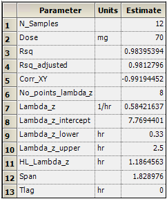
Part of the Final Parameters worksheet

Note the partial area estimates near the bottom of the Final Parameters.

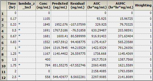
Click Summary Table in the Results list.

Note that values used in the calculation of Lambda Z are marked with an asterisk in the column Lambda_z_Incl. The data point corresponding to time 1.5, which was excluded manually, is not marked with an asterisk. The observation at time 2.0, with a value of zero, was automatically excluded.

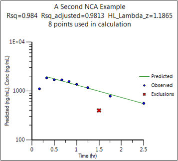
Click Observed Y and Predicted Y vs X.

The excluded data point is marked on the Observed Y and Predicted Y vs X plot output of observed and predicted data.

This concludes the partial areas example.