This section contains descriptions of the types of input data that can be used with the Phoenix Model object.
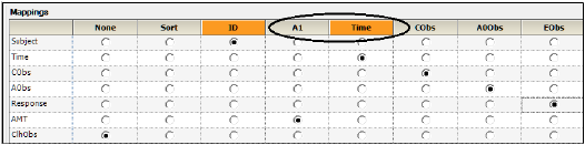
Phoenix NLME is extremely flexible on requirements for input data. There are no requirements for naming a variable as long as it is acceptable in a Phoenix spreadsheet (which does not allow special characters) and is not a reserved word for Phoenix NLME (see the previous Note). Column headers can contain any combination of alphanumeric characters and underscores. Once a spreadsheet is selected as an input to the Phoenix model, the user just has to 'map' the input column (listed in the left column) to the column expected by the system (listed in the top row). To specify a mapping, select a radio button in the row for the input column header under the corresponding column. The section below provides details and examples to illustrate how different data structures can be used in Phoenix NLME. This section refers to population analysis unless stated otherwise.
Note:The following are reserved words for NLME (case sensitive): cabs, hypot, chgsign, copysign, logb, nextafter, scalb, finite, pfclass, repl, isnan, j0, j1, jn, y0, y1, yn, UNI. Avoid using these words as names for variables. Similarly, refrain from using GNU reserved words (for a list of GNU reserved words, see gcc.gnu.org/onlinedocs/gcc-6.1.0/gcc/Keyword-Index.html).
Avoid special characters in the input data. Special characters, such as the Greek letter “beta,” in the data can cause NLME to abort execution.
Main Mappings panel input data
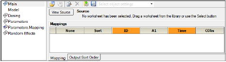
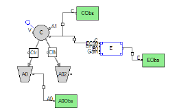
The Main Mappings panel under Setup is where the user should map most input data to be used by the Phoenix Model. When a Phoenix model is selected, the Main Setup tab displays the possible input data columns that can be used with the selected model. Required input is highlighted orange in the interface. As an example, for the default PK model that is shown when first opening a Phoenix model (one-compartment intravenous model with micro parameterization) there are 5 possible columns: Sort, ID, A1, Time and Cobs.
The number of columns may expand and column names may change depending on the model selected. The only variables names that cannot be changed are Sort, ID and Time. Columns highlighted in orange indicate that these variables are required by the model and names cannot be changed. For a PK model, these variables will be ID and Time, as illustrated below.
The following sections describe the different variables that may appear in the Mappings panel:
•Amount variables (e.g., A1, Aa, A1 Rate, A1 Strip)
When a column name is mapped as a Sort it indicates that the user wishes to do a subpopulation type of analysis. For each level of the sort variable the system will fit the same exact model (using the same model structure) but will output the results separated by sort level. For example, a column 'AgeGroup' could have the values of 'Young' and 'Elderly'. If that column is mapped as the sort, the same model will be fit twice: once to the 'Young' population and once to the 'Elderly' population. These independent fits will be presented in the same results spreadsheet and in the same graph outputs (different tabs) for easy comparison. The same results could be obtained by splitting the data between 'Young' and 'Elderly', running the same model on each of the subpopulations, and then merging the results and combining the plots.
Note that if the initial parameter estimates are entered in the model options in the bottom of the screen (see screen shot below), then each sort level model will use the same initial estimates.
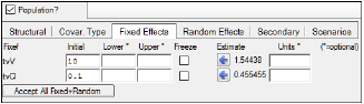
Initial estimates entered in Fixed Effects tab
On the other hand, if the user enters the initial parameter estimates using a worksheet under the Setup 'Parameters' option (either internal or external worksheet), then different initial estimates can be used per sort.
Note:If a variable is used as a sort it cannot be reused as a covariate within a model.
If there is more than one sort variable, the order for displayed results can be selected in the tab 'Output Sort Order'.
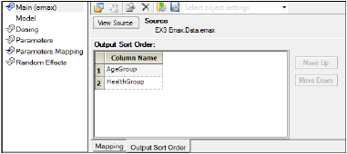
Output Sort Order tab
Columns mapped as Sort Variables can be character or numeric.
Input column(s) mapped as ID variable(s) identifies data items from the same individual within a population. The variable ID entries do not have to be numeric, increasing, consecutive nor unique.
The Phoenix NLME default setting of the checked option Sort Input? under Run Options will automatically sort the data by ID (up to 5 levels of ID) and then by Time (if the model is time-based). Unselecting this default option will process the data in the order given in the input dataset, and thus if the same subject ID is present in the dataset but the records are not consecutive they will be treated as two different subjects.
If a single ID entry within a column is non-numeric then the entire column is considered non-numeric, otherwise it is considered numeric. Note that non-numeric and numeric ID variables are sorted differently. For example, in numeric ID sorting, 2 comes before 10 but in non-numeric order 10 comes before 2.
If dosing information comes from a dosing worksheet (external or internal) then Sort Input? is automatically selected because of the need to merge the dosing and main worksheets. Similarly, if the model has a parameter worksheet that provides initial values, the 'Sort Input' option is automatically selected because it requires merging and thus sorting over sub-populations or individuals.
Note:If a non-population model is selected, the ID variable will disappear from the mappings and subject identification should then be mapped as a Sort instead.
If more than one ID column is mapped (i.e., a set of columns is required to uniquely identify data records from an individual) then the system provides the option of specifying the order of the ID columns. The Input Options tab displays all the ID variables with a bar to their right that allows the user to swap the order of ID pairs.
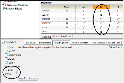
Note:The total number of ID plus SORT columns cannot exceed 5 variables.
Columns mapped as ID Variables can be character or numeric.
A time variable (i.e., independent variable) is required for time-based models (e.g. PK models, or any model capable of undergoing time-evolution). Columns mapped as Time must contain numeric values or character entries in an accepted time format.
The values in the Time column are evaluated to decide if time is complex or not. Time is considered to be complex if there is a Date column, or if the Time column contains anything indicating clock time, like a colon (:), “am”, “pm”, “a”, “p”, etc. If time is complex, it means time within the subject is measured relative to the first time in that subject, it is not absolute. If time is not complex (i.e., simple) it means time is absolute, so even if the first event in a subject occurs at time 10, the subject starts evolving at time 0, and evolves for 10 time units before getting to that first event.
If a dataset contains blank time data, the model will not execute.
|
Hour:minute:second format |
|
hh:mm:ss (24 hour clock, e.g., 15:00:00) |
|
hh:mm:ss tt (where tt can be 'am', 'pm', 'AM' or 'PM' in any mixture of upper and lower case, e.g., 03:00:00 pm) |
|
hh:mm:ss t (where t can be 'a','p', 'A' or 'P', e.g., 03:00:00 p) |
|
hh:mm (seconds are assumed 00, e.g., 15:00 or 03:00 pm or 03:00 p) |
This format (time with a ':' character) is converted into hours (basic unit of time) although no unit is printed in the output. If there are units in the time column these are not taken into account for this format.
Formats like hh:mm also accept non leading zeros so both 03:00 and 3:00 are accepted. Similarly, both 03:01 and 3:1 are accepted.
Hours are not limited to 24, and minutes and seconds are not limited to 60.
Hour or hour.fraction
Numeric times are accepted (integers and fractions). These can be used by themselves as relative times from first event, or in combination with a date variable. If they are combined with a date variable, then the dosing date/time will be subtracted from the sample date/time to calculate a relative time. For example, if the dose is given on 01/01/2010 at time 2 and the first and second samples are taken at 01/01/2010 at time 12.5 and 01/02/2010 at time 2 respectively, then the relative times used would be a dose at time zero and samples at times 10.5 and 24.
If there are units on a time column that contains numeric values without a date variable, these units are carried to the model output.
A Date format can be specified by checking the option of Date? and selecting an appropriate format in the Input Options tab. This option indicates that event times are a combination of a date and a time format. Note that when selecting a date format, the user needs to map two columns: one for date and one for time.
The accepted date formats in Phoenix NLME are:
•Day-Month-Year (most of world)
•Month-Day-Year (U.S.)
•Year-Month-Day (Asia, ISO)
•Year-Day-Month
The date consists of one, two, or three numbers separated by any non-numeric character (4 26 10, 2010/26/04, etc.). If there are three numbers, they are assumed to be the year, month, and day in whatever order the user has chosen. If there are only two numbers, they are assumed to be month and day. If only one number, it is assumed to be the day.
If the year is four digits long, it is taken as is. If the year is three digits long, it is assumed to be in the millennium starting at 1980. (000=2000, 979=2979, 980=1980). If the year is two or one digits long, it is assumed to be in the century starting at 1980. (99=1999, 00 or 0=2000, 79=2079, 80=1980). Leap years are assumed to occur in 1980 and every fourth year after. Leap seconds are not considered. If the year is not given, it is assumed to be 1980. This is the number called the “CenturyBase” and it is 1980, and cannot be changed in the User Interface although it can be changed in command-line mode.
Months are numeric, starting with 1 for January. If a month number is less than one or greater than 12, it is flagged as an error
Days of the month start with 1. If a day number is less than 1 or greater than 31, it is flagged as an error. The number of days in a month depends on the month, and for February, it depends on the leap year.
Dates are converted into the number of hours since 00 hours January 1, 1980.
A non-existent date, such as 1981/02/29 or 09/31 is not flagged, but just wraps into the following month.
Any combination of these time/date formats is accepted by Phoenix NLME.
Although Phoenix worksheets accept other date formats as input (see “Date and time formats”), only the four date formats above are accepted as time entries in Phoenix NLME.
Phoenix NLME does NOT require that time entries be sorted. By default, Phoenix NLME will sort the time entries within ID. This default can be overwritten by unselecting the Sort Input? selection under the Run Options tab (e.g., when executing pooled data models). If Sort Input? is unchecked, and time entries are not sorted in the input data, the model will not run.
Columns mapped as Time must be numeric values or text entries in an accepted time format. If the Date? option is selected, the user would then need to map both Date and Time columns in one of the accepted formats described above.
The variable 'C' is the independent variable for PD models (Emax and Linear models). Note that although this variable is not required by the system it is likely needed for modeling because if it is not mapped then it is assumed to be zero. Columns mapped as the independent variable C can contain character and numeric values. Numeric values can be negative and non-negative. Character values are treated as blanks (i.e., missing information) and therefore, values are backwards extrapolated if there is no prior information or forward extrapolated if there is prior information.
Phoenix model results (grids and plots) display the columns mapped to the 'C' variable as IVAR (“independent variable”).
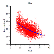
Example Phoenix Model plot
Columns mapped as independent variable 'C' can be numeric or character.
Amount variables (e.g., A1, Aa, A1 Rate, A1 Strip)
These variables represent amounts administered, stripping doses or associated rates of administration as applicable. The second letter usually indicates the compartment into which doses are being administered. Mapping this information in the Main tab is OPTIONAL, because it may also be mapped in the Dosing tab, or, if there are multiple dose routes, they need not all be used.
These variable names change depending on the library model selected. When using graphical or textual models the user can rename these variables.
For built-in (library) models the names of the columns representing the amounts dosed are as follows:
|
Name for Amount |
Definition |
Parameterization |
Type of Administration |
|
A1 |
Amount administered to Compartment 1 |
Micro, Clearance, or Macro |
Intravenous |
|
A1 Rate |
Rate of infusion |
Micro, Clearance, or Macro |
Intravenous or Infusion |
|
A1 Strip |
Stripping Dose |
Macro |
Intravenous, IV Infusion or Extravascular |
|
Aa |
Amount administered to the absorption compartment |
Micro, Clearance, Macro and Macro1 |
Extravascular |
|
A |
Amount administered to Compartment 1 |
Macro1 |
Intravenous or IV Infusion |
|
A Rate |
Rate of infusion |
Macro1 |
Intravenous or IV Infusion |
For example, when selecting a clearance model in which doses are given as intravenous infusions, the Main Setup mappings would automatically expand, allowing the user to optionally map A1 and A1 Rate.
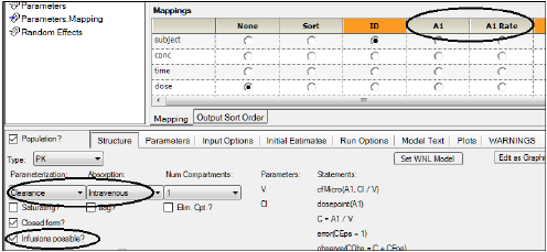
There are two types of macro-parameter models, denoted Macro and Macro1. They both are parameterized as a sum of exponentials, however, they differ in whether they directly model concentration (Macro) or amount (Macro1) in the central compartment. Thus, Macro models do not have a V (volume) parameter, while Macro1 models do have a V parameter.
Since Macro models use concentration, an assumption must be made about the size of a reference initial dose, called a “stripping dose”. Normally, this is taken to be the size of the actual initial dose, however, it can be overridden in the mappings panel.
The meaning of stripping dose: The Macro model has a sum of exponentials that are fitted to the original observed value of C, using some original dose, whatever it is. If the model is again fitted against data obtained at another time with a higher or lower dose, then the question is how to make the model predict higher or lower values of C. This is done by multiplying the model's predicted value of C by a ratio of the current dose and the original dose. The value used for the original dose is called the “stripping dose”, and it allows the model to be used with dose values and sequences different from the original. The Macro parameterization of Phoenix models is similar to the macro parameterization of the WNL5 models.
If no stripping dose is mapped on the Main or Dosing panels, the stripping dose is assumed to be equal to the initial given dose.
Note:It is not a requirement to map dosing information in the Main Setup tab. Dose can be mapped in the Main tab if dosing information columns exist in the dataset that contains the dependent variable. Otherwise, Phoenix NLME has other options for inputting dosing information as described in the Dosing Setup tab section in “Dosing panel”.
Macro1 parameterization is similar to other PK model parameterizations, in which the modeled quantity is amount A in the central compartment. The only difference is that A (not C) is modeled as a sum of exponentials. Macro1 models contain an additional volume V parameter, which converts amount A to concentration C, just as in the other PK models.
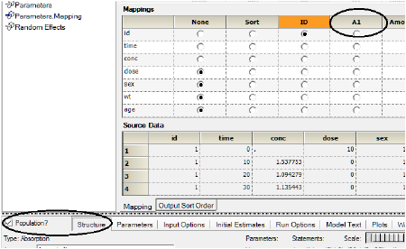
For pharmacokinetic models, if the dosing information is in the same dataset as time and concentration the dosing record has to be associated with the real time it was administered. As depicted below, in the table on the left doses are given at times 0, 0.5, 1, 3 and 6. In the table on the right dose is given only at time 0. Records can have a dose and an observation in the same row.
|
Subject |
Time |
Concentration |
Dose |
|
Subject |
Time |
Concentration |
Dose |
|---|---|---|---|---|---|---|---|---|
|
1 |
0 |
0 |
10 |
|
1 |
0 |
0 |
10 |
|
1 |
0.5 |
0.345 |
10 |
|
1 |
0.5 |
0.345 |
|
|
1 |
1 |
1.10 |
10 |
|
1 |
1 |
1.10 |
|
|
1 |
3 |
0.981 |
10 |
|
1 |
3 |
0.981 |
|
|
1 |
6 |
0.654 |
10 |
|
1 |
6 |
0.654 |
|
Columns mapped as Amounts, Stripping Doses or Rates can ONLY be numeric.
In the graphical editing mode, the user can provide their own name to amounts going into compartments as illustrated below.
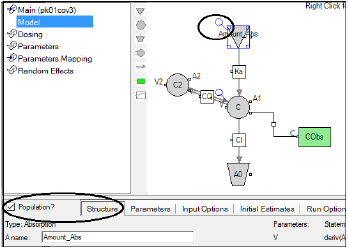
Context title updated to reflect user-entered name
In addition, amounts and rates can optionally have associated units. Details on units are listed under “Units labeling”.
There must always be a dependent variable in a model (i.e., the value of an observation). The default names for dependent variables in built-in models are CObs for PK models (i.e,. time-based models) and EObs for PD (effect) models, although these names can be changed by the user. If two or more records have the same Sort, ID, and independent variables (e.g., times) but different dependent variables (i.e., duplicate DV values) these entries are accepted by Phoenix as independent observations.
Values in columns mapped as dependent variables (e.g., CObs or EObs) can be character or numeric. Character and blank (i.e., missing) values are ignored by the model and thus, only numeric entries are taken into account. Negative and non-negative values are accepted.
Only numeric values in columns mapped as the dependent variable (e.g., CObs or EObs) are taken into account in a model.
Phoenix models can have multiple dependent variables. For example, a link or simultaneous PK/PD model would have PK observations and PD observations to model. Using a graphical model or a textual model allows the user to have more than two dependent variables in models. The names of the dependent variables used in models appear in the main mappings panel and the user is required to map at least one of them. The same data structure requirements apply to all the dependent variables where only the numeric values will be taken into account in the model.
Graphical model with two dependent variables
Dependent variables listed in the Main Mappings panel
Model covariates are selected in the Parameters/Structural tab (see “Parameters tab”). Covariates need to be mapped in the Main mappings panel. Failure to map a covariate that is needed in the model will result in a warning in the WARNINGS tab.
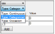
All covariates are assumed to be continuous unless the user selects a different covariate type (categorical or occasion) in the Parameters/Covar. Type tab.
All covariate values need to be numeric regardless of Type. This applies to columns mapped as categorical or occasion covariates. For example, gender should be 0/1 instead of Female/Male. The user can associate a label to the numeric categorical covariate and the label will be displayed in graphs even if the underlying data is numeric.
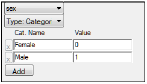
Numerical values assigned to categorical covariates
Columns mapped as covariates (including categorical or occasion covariates) can only be numeric.
Phoenix models can work with censored data. When the user checks the option BQL?, a new requirement is then to map a flag CObsBQL or EObsBQL in the main mappings panel.
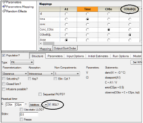
The CObsBQL or EObsBQL columns can contain two categories of values: nonzero (BQL) or 0/blank (normal non-BQL). If a concentration or response value is marked as BQL, then the cumulative distribution function evaluated at the corresponding value of CObs or EObs is used to calculate the likelihood, which is equal to the probability of falling into the interval between minus infinity to LLOQ, where LLOQ is given the value of the CObs or EObs column on that row. If a concentration or response value is flagged as non-BQL, then the probability density function is used to calculate the likelihood in the usual manner. The data tool 'BQL' provides a quick and easy way to create an observation column and its associated BQL flag column.
The engine automatically reverts to the Laplacian method when the BQL option is selected.
Only numeric values or blanks are accepted in columns mapped as the censoring flags CObsBQL or EObsBQL. A value of zero or blank indicates that the observation is NOT censored, and a nonzero numeric value (typically one) indicates the observation is censored.
