Phoenix allows a user to add their own columns, control which columns are needed in the model, and how they are mapped. The User-provided Extra Column Definition Text option can be used to assign the same column for two separate contexts in a model. For example, a PK model might require that the same concentration column be used in a model as the dependent variable as well as for a weighting. This extra column definition text is optional and can be used with built-in models when additional flexibility is needed to define mappings. If a user is modeling in textual or graphical modes, it is unlikely this option would be needed.
Another example of this option’s usability is to predefine some columns that do not exist in every dataset. By defining these columns, the same model can be run against different datasets. For example, one can define some dose regimens (using MDV, Reset, SS, ADDL, etc.) even if those columns do not exist in each dataset. The Phoenix engine will preprocess the data and a missing column will act like a column of missing data. In other words, the same model can be run against different datasets even if the dosing information is different by predefining some columns.
Several options are allowed in the Extra column definition field (Model Text > User-Provided Extra Column Definition Text). To define these additional columns, the user needs to type statements in the column definition syntax, which resembles PML (Phoenix Modeling Language) syntax but is much more restricted. If needed, the names of columns can be enclosed in double quotes (for example, for column names containing odd characters). In addition, the column assignment can be made using an equal sign (=) or using ‘<-’. Some examples of available statements are summarized below:
•id(columname): Can contain up to 5 identification column names separated by commas from least to most significant. Indicates the columns with IDs for a population.
•time(columnname): Indicates column containing time.
•obs(observedvariablename <- columname): Indicates column containing the observed variable.
•obs(observedvariablename <- columname, bql <-columnname): Indicates column containing the observed variable and the column with the flag for BQL (censoring flag).
•covr(covariatename <- columnname): Indicates variables that are covariates; as the default setting, these covariates propagate backwards in time or are interpolated.
•fcovr(covariatename <- columnname): Indicates variables that are covariates, but, in this case, these covariates propagate forward in time.
•date(columnname, optional format, optional century base): Indicates column with the time information formatted as a date. The accepted formats are ymd,ydm,myd,mdy,dym,dmy; century base is a four-digit year, like 1980, used to interpret two-digit years in the data.
•mdv(columnname): Indicates the MDV column.
•dose(dosepointname <- amountcolumnname) or dose(dosepointname <- amountcolumnname, ratecolumnname): Indicates the amount column to be mapped to each dosepointname and optional rate column (for infusions). There are several options to indicate multiple doses given to the same dosepoint name. The user is referred to the “Column mappings” for the PML syntax of these advanced specifications.
•reset(columname) or reset(columname, value) or reset(columname, c(lowvalue, highvalue)): Indicates that there is a reset event and specifies the column that triggers it.
The idea of Reset is that a subject could go through a time-sequence of doses and observations with time starting at zero typically, and then go through another like it, starting from zero, independent of the first sequence, but the same etas would apply to the entire subject. Therefore, the data cannot be sorted if Reset is selected and the first row of data for the second and subsequent sequences would have the reset flag. The subject's state is reset, including compartments and any other integrators, sequence statements, any outstanding infusions or delayed doses, before anything else on that row happens: dose, observation, or covariates. See “Simple versus complex time” for additional information.
Writing an extra column definition statement that assigns a column name to a function in the model does not automatically show this additional extra column in the Main mappings panel, Thus, the user needs to verify that the column defined (following the “<-” or “=” sign) indeed exists in the input dataset.
Columns mapped as a User-Provided Extra Column Definition can be numeric or character depending on how they are used in the model.
When using Reset, it is important to understand the two kinds of time, simple and complex.
•Time is complex if any value in the time column has the appearance of clock time, such as by containing a colon(:) character, as in hours:minutes, or if it contains AM or PM, or if there is a date column.
•Time is simple if there is no date column, and if every time value is a simple decimal number.
If time is simple, the first record for a subject represents absolute time since zero. For example:
ID TIME AMT
100 6.5 10
means that subject 100 is initialized (which includes starting sequence blocks), and then is evolved for 6.5 time units before the dose of 10 is administered.
Similarly, if there is a Reset row:
ID TIME AMT RESET
100 … … …
100 6.5 10 1
it does not mean the subject is reset at time 6.5. It means the subject is initialized (including sequence blocks), and then is evolved for 6.5 time units before the dose is administered. The only thing retained about the subject is its parameter values.
If time is complex, that means it is an arbitrary clock time, not an absolute time relative to some origin. For example:
ID TIME AMT
100 6:30 10
means that subject 100 is initialized (which includes starting sequence blocks), and then is evolved for zero(0) time units before the dose of 10 is administered.
Similarly, if there is a Reset row:
ID TIME AMT RESET
100 … … …
100 6:30 10 1
it does not mean the subject is reset at time 6:30. It means the subject is initialized (including sequence blocks), and then is evolved for zero(0) time units before the dose is administered. The only thing retained about the subject is its parameter values.
Parameters and parameter mappings
Fixed effects initial estimates for modeling or fixed effects estimates for simulation should be entered in the models. This section explains the data structure for these estimates, which will be referred to as initial estimates, although they might also be fixed effects parameter estimates for simulation.
There is more than one way to enter initial estimates for a model:
-
Same initial estimates apply to all the sort variables (e.g., same initial estimates for all subjects when doing individual modeling):
•Type the initial estimates (and bounds) in the model specification (Parameters > Fixed Effects tab).
•Use the Initial Estimates tab to visually determine a set of parameter estimates that approximate the data and accept those estimates as initial estimates which are placed in the Parameters > Fixed Effects tab.
-
Initial estimates can be provided for each individual sort by typing in the information or using a file that contains that information:
•Enter information in the Parameters Setup grid.
•Map the information in the Parameters Setup Mappings panel.
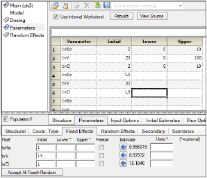
This section discusses data structure requirements for Method 2. The Parameter Setup grid allows the user to enter the name of the parameter, the initial estimate, the lower bound, and the upper bound.
When using an internal worksheet, the Sort values and Parameter names will be picked up from the model. The requirements for initial estimates and bounds are that they be numeric values.
Entering or mapping values in the Parameter Setup grid will overwrite any other values that might have been entered in the Parameters > Fixed Effects tab. In addition, if only partial information is entered in the Parameters grid (i.e., if some estimates are blank) the program will use the estimates from the previous profile in the Parameter Setup grid. In other words, if any information is entered in the Parameter Setup grid, then none of the estimates in the Fixed Effects tab will be used. In the example depicted below for individual modeling, Subject 1 will have initial estimates for tvKa, tvV and tvCl of 2, 20, and 2 respectively (plus entered bounds), Subject 2 and the rest of the subjects will be assigned initial estimates of 1.5 (tvKa), 22 (tvV), and 1.5 (tvCl).
If an external worksheet is selected, then a Parameter column should exist in the dataset and, optionally, numeric columns for Initial estimates, Lower bounds, and Upper bounds. The names of these columns are irrelevant as they get mapped to the corresponding location. There are no restrictions on the values for the parameter names in the column mapped to the Parameter column. The association of parameter names needs to be made in the new Parameters mappings panel that is displayed when entering Parameters from an external worksheet.
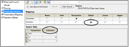
Initial context mapped to existing column in the source data
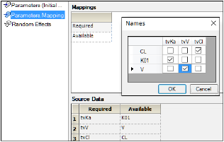
The Parameter.Mapping grid allows the association of any name of a parameter with the expected parameter name from the specified model. This association can be made manually, although the tool will try to automatically match names that are exactly the same.
Initial estimates and bounds need to be numeric values. Entering or mapping values in the Parameter Setup grid will overwrite any other values that might have been entered in the Parameters > Fixed Effects tab.
Phoenix allows the user to label the model parameters (primary as well as secondary) with units. These units do not play a role in the model fitting and there is no conversion that takes place.
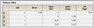
When an input dataset has the pertinent columns with units that define units for the model parameters (e.g., for a PK model without covariates: time, concentration and dose), then these units are carried to the output for fixed effects and secondary parameters. In this case, the user is not allowed to enter different units when specifying the model. The units for each column need to be part of the header for Phoenix to understand them as units and carry them forward to the model results. Note that as long as there is text in the unit location, it will be used as unit labels for the fixed effects and secondary parameters. Other Phoenix tools require that the units are valid (as denoted by being between parentheses) to perform unit transformations, but this is not a requirement for Phoenix models as these are merely used as labels.
If the input dataset has no column units, then the user can optionally enter the units for each of the fixed effects as well as secondary parameters. These fields do not have any specific requirement as they are used as labels.
There are no requirements for the units as they are used as labels, but it is a good practice for the user to make sure that the units make sense within the dataset (e.g., the concentration mass unit is the same as the dose unit) and that the initial estimates are provided in the expected units. The Data Wizard can be used to do any unit transformation prior to modeling. See the “Data Wizard” description.
It is recommended that the input dataset be consistent with regard to units that define the model parameters. In other words, data values should preferably be in the same mass, time, volume, etc. units.
