This section describes the requirements for variables selected in the Input Options tab that are related to the dosing regimen, which can be mapped in either the Main mappings panel or the Dosing mappings panel. Other common variables between the Main mappings panel and the Dosing mappings panel follow the same data structure described above.
Phoenix provides great flexibility for entering dosing regimens through the use of MDV, Steady State, ADDL and their associated options.
The MDV flag indicates that there is a missing dependent variable. This flag is optional for Phoenix models as the tool recognizes which records contain observed values and which do not. However, it can be optionally used, for example, to exclude observations from certain analyses.
The MDV flag needs to be numeric or blank, with nonzero numeric values indicating that the dependent variable value is treated as missing (typically a value of one is used), and zero values or blanks indicating that the dependent variable value is present.
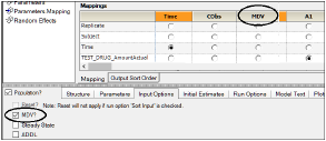
The user can indicate that a column of MDV flags is needed by checking the MDV option in the Input Options tab. This action will add a new column mapping, MDV, in the Main and Dosing mappings panels. Any column name can be mapped to MDV but the program will map it automatically if the exact column name of ‘MDV’ is in the worksheet.
To summarize, the rules that determine which records are used in Phoenix NLME are as follows:
•If a single data sheet (combined dosing and observations) is mapped from the Main panel and if a dose and a nonzero observation appear on the same line, then the nonzero observation is treated as real data and is not ignored (except if there is an explicit nonzero MDV entry on the line, in which case the observation is always ignored). If a dose and an observation of 0 appear together on the same line, then the observation is ignored.
•If the dosing information is mapped from the Main panel, and if there is no associated dose record, and if there is no MDV entry or no MDV entry greater than zero, then an observation with a value (including a value of zero) is a valid observation.
•If the dosing information is entered using the dosing panel (either by entering it manually in an internal worksheet or obtaining it from a file containing dosing information), then the dosing information is not merged in the same line as the observation information even if the time entries are the same. In this case, all the observations will be used unless there is an explicit nonzero MDV flag on the observation line.
The steady-state flag indicates whether the associated dose is a steady-state dose. When an observed dose is flagged as a steady-state dose, this dose is assumed to have been preceded by a series of dose cycles given at certain regular time intervals such that they have reached steady state (i.e., PK equilibrium). The doses preceding the observed dose have not been captured in the dataset and thus the information has to be entered. The steady-state flag and the 'implied' dosing information indicate to Phoenix that the formulas to be used need to compute the steady-state amounts at the time the steady-state dose is introduced.
The steady-state flag needs to be numeric:
•Values of zero or blank indicate that the record is simply an ordinary dose.
•Values greater than zero indicate that prior to giving the indicated dose, the PK model is put into steady state.
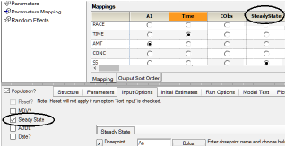
The user can indicate that steady state is possible by checking the Steady State option in the Input Options tab. This action will add a new column in the Main and Dosing mappings panels called SteadyState. Any column name can be mapped to SteadyState but the program will map it automatically if the exact column name of 'SteadyState' exists in the external worksheet.
When a record is flagged as being at steady state the program needs some additional information about the dosing cycle when this steady-state observation was taken. The additional information needed is the dose given (Amount), the time interval between doses (Delta Time), and the mode of administration and the compartment that received the dose (Dosepoint). In addition, the dosing cycle can consist of multiple doses such as AM and PM doses.
When the Steady State flag is checked under the Input Options tab, a Steady State sub-menu for entering the additional dosing information will be displayed.
•Dosepoint: This information consists of two parts; the mode of administration (either bolus or infusion) and the dose name and the compartment in which the dose is administered (e.g., default name 'Aa' for a one-compartment oral administration). The dosing variables section describes the default names for the built-in models. See “Dosing panel”. The user must enter this dosepoint name, and thus the name needs to exist in the model. All available dosepoint names will be listed in the Main mappings panel.
•Amount: the dose amount given at each time interval during the cycle. If the amount can be entered manually and is assumed to be constant during a dosing cycle, then the Constant button should be selected and the dose amount entered. If the dosing cannot be assumed to be constant or the user wishes to enter it from a file, then click on the toggle button and select Column and enter the name of the column that contains this information.
When entering the steady-state amount from a column, no additional mapping column is displayed with this option. The user needs to be sure that this column (containing steady-state dose amounts) indeed exists in the input dataset that contains the dose information for the observed record.
Constant amounts entered or from columns containing amount values should be numeric and positive.
•Rate: If the dosepoint route of administration is selected as an Infusion, then a rate of infusion needs to be provided. This rate should be a positive numeric value and the units should be in accordance to time units in the input dataset.
If the rate of infusion is assumed to be constant during a dosing cycle then the Constant button should be selected and rate entered in the field. If the rate cannot be assumed to be constant or the user wishes to enter it from a file, then click on the toggle button to select Column and enter the name of the column containing this information.
When entering rate from a column, no additional mapping column is displayed with the name of the rate column, and the user needs to ensure that this column (containing rate of infusion) indeed exists in the input dataset that contains the dose information for the observed record.
Constant amounts entered and entries in columns containing rates of infusion should be numeric and positive.
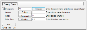
•Delta Time: the time interval between doses that allowed steady state to be reached. If the elapsed time between 'implied' doses can be assumed constant during a dosing cycle then the Constant button should be selected and the time interval typed in the field. If the delta time cannot be assumed constant or if the user wishes to enter it from a file, then click on the toggle button to select Column and enter the name of the column that contains this information.
When entering steady-state delta time from a column, no additional mapping column is displayed with this option and the user needs ensure that this column (containing steady-state delta time) indeed exists in the input dataset that contains the dose information for the observed record.
Constant delta time entered and entries in columns containing elapsed time between doses should be numeric and positive.
The dosing cycle can contain multiple steps and doses to multiple compartments. This is specified by adding segments to the cycle, by clicking the Add button. The total length of the cycle is the sum of the Delta Time parts of each segment. In steady state, in each segment of the cycle, the dose occurs first, followed by the delta time.
Only numeric values or blanks are accepted in columns mapped to SteadyState. A value of zero or blank indicates that the observation is NOT collected at steady state. Any other value indicates that the model is put into steady state before administering the dose on that row.
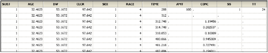
Example: The selections for steady state depicted below indicate that an infinite number of bolus doses are assumed to have been added to the amount in the absorption compartment in the model (Aa) for that subject, in the amounts provided in the AMT column in the dataset, at time intervals provided in the TT column in the dataset. Therefore, for Subject 1, the data are assumed to have been collected at steady state following a dosing regimen of 100 oral units every 24 hours, with the most recent dose administered 24 hours ago.
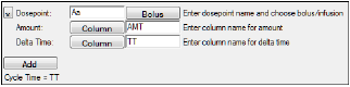
Example selections for steady state
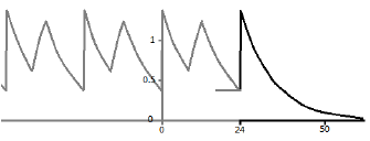
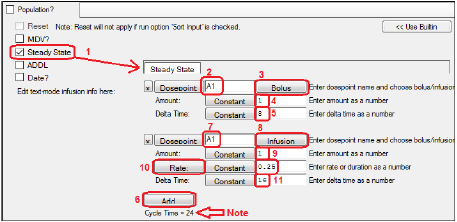
More complex example: Suppose the volume of a 1-compartment model is 1. Suppose it is desired to say that at time 24, one can assume there has been a continuous series of dosing cycles taking place, where the cycle consists of first a bolus dose of 1 unit, and then 8 hours later a 4-hour infusion of 1 unit is given. Then the next cycle starts 24 hours after the initial bolus. Also suppose at time 24 a single bolus of 1mg is given.
The following plot shows concentration versus time. Notice that at time 24, when the actual dose is given, the prior concentration is not zero. It is about 0.4, because of the prior assumed dosing cycles, shown in light gray.
This situation is set up as follows:
-
On the Input Options tab, check the Steady State option to display the Steady State sub-tab.
-
Enter the name of the dosepoint to receive the dose, if necessary (e.g., A1).
-
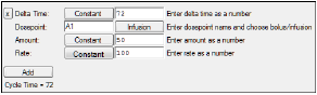
Set up the initial bolus by making sure the Bolus/Infusion option is set to Bolus.
-
Enter the amount of the dose (e.g., 1 unit).
-
Enter the wait time before the next dose (e.g., 8 time units).
-
Click the Add button to enter the second dose.
-
Enter the name of the dosepoint (which does not have to be the same as the prior dosepoint).
-
Make sure the Bolus/Infusion button says Infusion.
-
Enter the amount of the infusion (e.g., 1 unit).
-
Make sure the Rate/Duration button says Rate and enter the rate (e.g., 0.25 drug units per time unit).
-
Enter the time that passes before the cycle repeats (e.g., 16 time units).
Note the total cycle time appears below the Add button.
The concentration-time curve in the graph shown earlier in this section arose from the following dosing input:
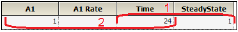
This says two things:
•At time t=24 the model is put into steady-state, on the assumption that the dosing cycle above occurred at t – 24, t – 48, etc., but not at time t.
•A bolus dose of 1 unit is given at time t.
Note that the delta-time comes after the dose. The reason for this is that the dose may be an infusion; it may have a tlag; it may be zero-order (implied infusion). These delayed aspects of the dose have to be completed before the dosing cycle completes. This might be considered a limitation of the software, but it is necessary to assume that if a subject is in steady-state prior doses have actually completed.
ADDL can be regarded as a number of additional dose(s) that were not observed but were administered. For example, this can be used to indicate that additional doses will be given after the observed dose.
ADDL can only take positive numeric values as it represents the number of additional doses given. Additional dose information needs to be provided and will be applied each time to the number of additional doses indicated by the ADDL record.
The user can indicate additional doses were received by checking the ADDL option in the Input Options tab. This action will add a new column in the Main and Dosing mappings panels called ADDL. Any column name can be mapped to ADDL, but the program will map it automatically if the exact column name of 'ADDL' exists in the external worksheet.
When ADDL is checked under the Input Options tab, an ADDL sub-menu for entering the additional dosing information will be displayed. The information requested will be the Dosepoint (mode of administration and the compartment it was given to), the amount, the rate if an infusion was administered, and the time interval or delta time between doses. The data structures for these options are exactly the same as described in the steady-state section above. However, there is one major difference between ADDL and Steady State, even though the data structure requirements are the same. In Steady State, the dose occurs first, followed by the delta time; in ADDL, the delta time occurs first, followed by the dose.
Only numeric values or blanks are accepted in columns mapped to ADDL. A blank value is ignored; a positive numeric value indicates the number of additional doses given, which need additional information, namely, Dosepoint, Amount and Delta Time.
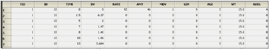
Example: The screen shot below is an ADDL, set up to simulate a dosing regimen. For Subject ID 10, the simulated regimen consists of four infusions of 50 mass units at a rate of 100 mass units per time unit (i.e. duration=0.5 time units) every 72 time units (e.g., hours), starting at time zero.
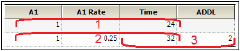
More complex example: Suppose a bolus dose of 1 unit given at time 24 (area 1 in the “Concentration vs. Time plot”), followed by a 4-time-unit infusion (area 2) started at time 32 (8 hours after the bolus), followed by two additional cycles (areas 3 and 4) just like it.
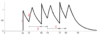
The additional cycles have to start at the time of the last actual dose, which is the infusion that starts at time 32. So the cycle, as depicted in area 3 for example, starts with an initial delay of 16 time units, then the bolus, then a delay of 8 time units, then the start of the next infusion. This cycle is repeated as many times as requested, in this case 2 times.
-
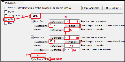
On the Input Options tab, check the ADDL option to display the ADDL sub-tab.
-
Click the Add button.
Notice how ADDL differs from the Steady-State user interface. The Delta Time delays come first. -
Enter the initial delay (e.g., 16 time units).
-
Enter the name of the dosepoint to receive the dose (e.g., A1), if necessary.
-
Make sure the Bolus/Infusion option is set to Bolus.
-
Enter the amount of the dose (e.g., 1 unit).
-
Click the Add button to enter the second dose.
-
Enter the initial delay (e.g., 8 time units).
-
Enter the name of the dosepoint (which does not have to be the same as the prior dosepoint).
-
Make sure the Bolus/Infusion button says Infusion.
-
Enter the amount of the infusion (e.g., 1 unit).
-
Make sure the Rate/Duration button says Rate and enter the rate (e.g., 0.25 drug units per time unit).
Note that the total cycle time is shown below the Add button.
Settings for complex ADDL example
The concentration-time curve shown in the “Concentration vs. Time plot” arose from the following dosing input:
Dosing input
This says three things:
•A simple bolus of 1 unit occurs at time 24.
•A 4-time-unit infusion begins at time 32 (8 hours after the bolus).
•Two of the ADDL cycles begin at time 32.
Since the first cycle begins with a 16-time-unit delay, it means that the bolus in the cycle occurs at time 48, which is 24 hours after the initial bolus called for in the data.
Specifying steady state and additional doses outside of the user interface
Steady state dosing can be specified outside of the user interface. Consider the following data from an input file.
|
id |
time |
SSOffset |
A1 |
Aa |
SS |
II |
|
1 |
0 |
|
100 |
30 |
1 |
8 |
|
1 |
0 |
3 |
50 |
60 |
2 |
8 |
The column definition text file contains these lines:
sscol(SS)
iicol(II)
ssoffcol(SSOffset)
where sscol(SS) indicates that there is a column named SS (meaning steady state), and iicol(II) indicates that there is a column named II (meaning interdose interval). The SS column contains values 1 or 2 (or nothing). Note, rows in which SS is 2 can only follow rows in which SS is 1 or 2.
When the first row is encountered, at time 0, it means that the model will undergo a cycle of II time units (in this case 8), where each iteration of the cycle consists of a dose of 100 to A1, and a dose of 30 to Aa, followed by 8 hours until the next repetition. This cycle is conceptually repeated sufficient times to bring the model to steady state, ending at time 0, because 0 is the time on the row. Then, at that time, the doses are repeated one more time.
Multiple cycles can be superimposed, as shown by the second row, in which SS is 2, indicating an 8 time-unit cycle with a dose of 50 to A1 and 60 to Aa. However, the doses are not given at time 0. They start at time 3, because there is a datum 3 in the SSOffset column. So the cycle looks like this:
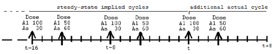
Illustration of steady state cycle
Up to nine SS=2 rows can follow an SS=1 row. In addition, the interdose interval (II) values do not all have to be the same. However, the least common multiple of the interdose intervals must not be more than ten times the longest one. This prevents combinations of interdose intervals like 24 and 23 (for which the least common multiple would be 552 time units).
Note on transferring NONMEM datasets to NLME, and vice-versa: In the case that a NONMEM dataset contains rows in which SS=2, and in which the time value on that row differs from the SS=1 row above it, it is necessary to introduce an additional column for SSOffset:
|
id |
time |
A1 |
SS |
II |
|
1 |
10 |
100 |
1 |
12 |
|
1 |
13 |
50 |
2 |
8 |
|
1 |
16 |
50 |
2 |
8 |
Note the different values in the time column.
|
id |
time |
SSOffset |
A1 |
SS |
II |
|
1 |
10 |
|
100 |
1 |
12 |
|
1 |
10 |
3 |
50 |
2 |
8 |
|
1 |
10 |
6 |
50 |
2 |
8 |
Note the same values in the time column with the additional offset column data (SSOffset).
This was necessitated by the Sort option on input data.
Additional doses can be specified as follows:
|
id |
time |
A1 |
Aa |
II |
ADDL |
|
1 |
0 |
100 |
30 |
8 |
10 |
|
1 |
3 |
50 |
60 |
8 |
10 |
The column definition text file contains these lines
addlcol(ADDL)
iicol(II)
where addlcol(ADDL) indicates that there is a column named ADDL (meaning additional), and iicol(II) indicates that there is a column named II (meaning interdose interval).
When the first row is encountered, at time 0, first the doses into A1 of 100 and Aa of 30 are performed, and then 10 more of those doses are scheduled into the future, at 8 time-unit intervals, because ADDL=10 and II=8.
Then, when the second row is encountered at time 3, first the doses into A1 of 50 and Aa of 60 are performed, and then 10 more of those doses are scheduled into the future, at 8 time-unit intervals.
Together the ADDL doses look like this:
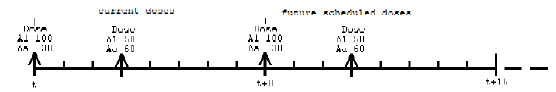
Illustration of additional doses
SS and ADDL dosing may be combined, as in the following:
|
id |
time |
SSOffset |
A1 |
Aa |
SS |
II |
ADDL |
|
1 |
0 |
|
100 |
30 |
1 |
8 |
10 |
|
1 |
0 |
3 |
50 |
60 |
2 |
8 |
10 |
where the column definitions are:
sscol(SS)
iicol(II)
ssoffcol(SSOffset)
addlcol(ADDL)
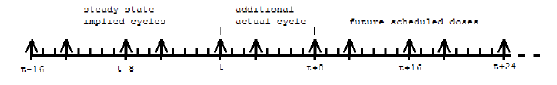
Illustration of combined steady state and additional doses cycle
Covariates may be included on SS or ADDL lines, but observations will be ignored.
