The Parameters tab contains six sub-tabs that allow users to modify the structural parameters, specify values for the fixed and random effects, and add covariates.
![]() Covariate effects can be specified in individual modeling, however, care must be taken not to over-parameterize the model. For example, suppose body weight W affects volume V. Then the model for V might be V=tvV+W*dVdW. In this case, if W is constant for the individual, the model is over-parameterized, because tvV and dVdW are redundant. However, if W is time-varying, the model is not over-parameterized.
Covariate effects can be specified in individual modeling, however, care must be taken not to over-parameterize the model. For example, suppose body weight W affects volume V. Then the model for V might be V=tvV+W*dVdW. In this case, if W is constant for the individual, the model is over-parameterized, because tvV and dVdW are redundant. However, if W is time-varying, the model is not over-parameterized.
Other covariates can be included in the individual model, even though they may not affect any structural parameters, because they may appear in secondary parameters, such as AUC.
The Structural tab lists all the structural parameters used in the model. The listed parameters change depending on the selections made in the Structure tab.
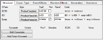
Structural Parameters tab for Emax model
Every selection made in the structural tab changes the code for the modified structural parameter. These code changes are displayed in the Model Text tab.
-
Click the buttons below Style multiple times to toggle through the different style options for each structural parameter: Sum+eta, Product*exp(eta), Sum*exp(eta), exp(Sum+eta), ilogit(Sum+eta).
The most common recommended form is Product*exp(eta) for positive-only parameters like V, CI, or various Ks. For parameters like E0 or Emax, which can be positive or negative, Sum+eta is the preferred choice, For parameters that are constrained to fall between zero and one, ilogit(Sum+eta) is a useful choice.
If there are no covariates, Product*exp(eta) and Sum*exp(eta) yield nearly identical expressions in the model code. The differences between the two are seen when there are covariates and they come into the equation either through multiplication or addition. For example, here is what Product*exp(eta) provides in the presence of covariate effects, where the user has chosen V and Cl on Gender, wgt, and apgr:
stparam(V=tvV
*(wgt/mean(wgt))^dVdwgt
*(apgr/median(apgr))^dVdapgr
*exp(dVdGender1*(Gender==1))
*exp(dVdGender2*(Gender==2))
*exp(nV)
)
stparam(Cl=tvCl
*(wgt/mean(wgt))^dCldwgt
*(apgr/median(apgr))^dCldapgr
*exp(dCldGender1*(Gender==1))
*exp(dCldGender2*(Gender==2))
*exp(nCl)
)
Here is what Sum*exp(eta) gives you in the presence of covariate effects:
stparm(V-(tvV
+(wgt-mean(wgt))*dVdwgt
+(apgr-median(apgr))*dVdapgr
+(Gender==1)*dVdGender1
+(Gender==2)*dVdGender2
)
*exp(nV))
stparm(Cl=(tvCl
+(wgt-mean(wgt))*dCldwgt
+(apgr-median(apgr))*dCldapgr
+(Gender==1)*dCldGender1
+(Gender==2)*dCldGender2
)
*exp(nCl))
-
In the Fixef field type a name for the fixed effect or use the default (tv (typical value)+the parameter name (tvV, tvKe, etc.)).
-
Check the Ran checkbox beside each parameter to add a random effect to the structural parameter (the parameter is added to the Random Effects tab).
-
In the Ranef field, type a name for the random effect or use the default name (n (eta)+the parameter name (nKa, nV, nKe, etc.)).
The bottom section of the Parameters’ Structural tab allows users to add covariates to the model structure. There are no covariate effects in individual modeling. Covariates are used because some secondary parameters like AUC depend on them. Covariates can be useful if the data are pooled, or all subjects are modeled together.
 -
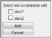
Click Add Covariate to add a covariate or click Add From Unused to add a covariate from the main input dataset.
A list of all variables mapped to None in the Main Mappings panel is displayed.
-
Turn on the checkbox beside each variable to add as a covariate.
-
Click Add to add the variable(s) as covariates or click Cancel to exit the Add From Unused Columns menu without adding any covariates.
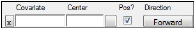
Covariate settings
To remove a covariate from the model, click the corresponding X button.
-
In the Covariate field enter a name for the covariate or use the default.
-
In the Center field, type the centering value for the covariate or click the
 button following the field to toggle between entering numeric value, using the mean, or the median.
Only continuous covariates can have a center value. See “Covar. Type tab” for instructions on selecting the covariate type. -
Clear the Positive? checkbox if the covariate values are not all positive.
-
Click Direction to specify the method of curve fitting if the covariate value changes between observations for a subject.
-
Click Forward multiple times to toggle through the curve fitting methods:
•Forward holds the first value between covariate observations.
•Interpolate linearly interpolates the covariate between covariate observations. Only available for Continuous covariate types.
•Backward holds the last value between covariate observations.
Covariates can also be added based on available columns in the input source. See “Considerations when modeling with covariates” for additional information on covariate direction.
-
Under each structural parameter there is a button to indicate how a given covariate can effect that structural parameter. The default is No (no covariate effect). Click the button multiple times to toggle through the other two options: Yes and 1+. The 1+ option is only available for Product*exp(eta) structural parameters, and is not the recommended choice.
Adding covariate effects to structural parameters
Users can add three types of covariate effects to structural parameters. They are continuous, categorical, and occasion. Each type has its own set of options, and affect the structural parameters and the model differently.
The structural parameters are displayed beside each covariate that is added.
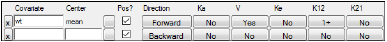
Covariate settings with structural parameters displayed
Each time a covariate effect is added, the code in the Structural tab and in the Model Text tab is modified.
Continuous covariate effects
Each parameter has a button that toggles between three values as it is clicked: No (the default), Yes, +1. The value shown on the button when the object is executed defines how covariate effects are added to structural parameters.
-
No does not add covariate effects to the parameter.
-
Yes adds covariate effects to that parameter by updating the code with an additional term
For example, if the effects of the covariate wgt are added to the structural parameter V, a new fixed effect parameter is created called dVdwgt and the term wt^dVdwgt is added). dVdwgt is also added to the Fixed Effects tab, and users can enter initial, lower, and upper values for the fixed effects parameter, In this example, dVdwgt is the derivative of the parameter value with respect to weight. dV is the increment of volume divided by dwgt, the increment of weight. -
+1 also adds covariate effects to the parameter by updating the code with an additional term (e.g., for the covariate wgt added to the structural parameter V, the term 1+wt*dVdwgt is added).
Each covariate effect added creates a new fixed effect in the Fixed Effect tab. The new fixed effect can be modified in the same way as any other fixed effect.
Categorical covariate effects
Each parameter has a button that toggles between three values as it is clicked. The value shown on the button when the object is executed defines how covariate effects are added to structural parameters.
Users cannot enter center values for categorical covariates.
-
No does not add covariate effects to the parameter.
-
Yes adds covariate effects to that parameter by updating the code with an additional term
-
+1 also adds covariate effects to the parameter by updating the code with an additional term.
Each covariate effect added creates a new fixed effect in the Fixed Effect tab. The new fixed effect can be modified in the same way as any other fixed effect.
Occasion covariate effects
The occasion covariate effect is used in a different way for variables. For example, the occasion could specify whether or not an observation was taken on a Monday or a Wednesday.
Each parameter has a button that toggles between two values as it is clicked. The value shown on the button when the object is executed defines how covariate effects are added to structural parameters.
-
No does not add covariate effects to the parameter.
-
Yes adds covariate effects to that parameter by updating the code with an additional term.
Adding an occasion covariate creates a copy of each selected structural parameter random effect in the Random Effects tab. For example, if V is a structural parameter, and an occasion covariate is added to it, then nV is added to the Random Effects tab, where n stands for eta, or random effect, and V stands for volume. If three occasion covariate effects are added for V, they are named nV, nV2, and nV3.
The new random effect can be modified in the same way as any other random effect.
Considerations when modeling with covariates
Covariates may have apparent incorrect covariate values being propagated (contrary to observed data), because of forward/backward/interpolate, for time-varying covariates. This raises several significant issues to consider when modeling:
-
It is important to note that covariates have a direction of propagation which is forward in time, backward in time, or linearly interpolated.
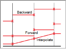
Illustration of propagation direction
The default is forward in time, to be somewhat consistent with other tools. (Refer to “Structure tab” for setting the direction.)
-
The propagation occurs over records with missing covariate values, which is not consistent with some other tools. The user needs to be aware that if an observation has a missing covariate value the covariate will take on a propagated value, rather than a zero value.
Note:In situations where a covariate is completely missing because it has not been mapped, Phoenix NLME exits with an error message. If the covariate is mapped, but one or more subjects do not have a row of data for that covariate, Phoenix NLME also exits with an error message. For example, if one subject did not have the variable “gender” at all and the model includes “gender” as a covariate for V, for instance, then the full model will fail.
There is no concept of a default value for a completely missing covariate, missing rows of data need to be resolved in the dataset prior to modeling.
-
In a table definition, one of the options is When Covr. Set. If two covariates are specified in this field, and if they are both set to new values at the same time, one of them is actually set before the other, even though they are both at the same time. A row is added to the table for each covariate setting, so only the second row will contain the new values for both covariates. This extends to multiple covariates named in that field. A workaround is to figure out which covariate is set last (should be the last one declared in the model), put just that one in the When Covr. Set field, and include other covariates in the Variables field. (Refer to “Simple run mode table options” for setting these options.)
Regardless of covariate direction, the value of the covariate applies during all other dose or observation events occurring on the same input data row. For example, if the data looks like this:
time CObs age weight
...
14 99.7 17 50
...
If there is any doafter code associated with observable CObs, the age and weight have the value 17 and 50 in that code, regardless of forward or backward covariate direction.
The Covariate Type tab allows users to specify covariate types. The default setting for each covariate is Continuous.

-
In the top, unlabeled menu, select the covariate.
-
In the Type menu, select the covariate type: Continuous, Categorical, Occasion.
If Categorical is selected, users can enter values for the categories. A minimum of two categories is required for categorical covariates.
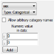
•In the Numeric value in data field, type a value for each category. It is typically best to use consecutive integers, starting at zero.
•If the Allow arbitrary category names checkbox is checked the user is able to specify a name for each category and enter an associated value. The categorical values entered must be in the main input dataset.
Note that the actual text values that were in the dataset will appear in the Settings output and History to clarify the mappings that were set (e.g., covr(Gender<-”TextGender”(Male=0, Female=2))).
•To add another category, click Add.
•To remove a category, click the corresponding X button.
If Occasion is selected, users can enter values for the dosing or observation occasions. A minimum of two categories is required for interoccasional covariates (refer to “Setting up interoccasional covariates”).
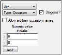
•In the Numeric value in data field, type a value for each occasion.
•Check the Allow arbitrary occasion names checkbox to specify a name for each category and enter an associated value. The occasion values entered must be in the main input dataset.
•To add another dosing or observation occasion, click Add.
•To remove a dosing or observation occasion, click the X button.
•Use the Diagonal? checkbox to set the interoccasion covariance to a diagonal structure (box is checked, this is the default) or block structure (box is unchecked).
![]() Occasion covariates are always available but they are only used with population models. They are not used with the individual models that Phoenix processes. Using occasion covariates with individual models has no effect on the model or the output.
Occasion covariates are always available but they are only used with population models. They are not used with the individual models that Phoenix processes. Using occasion covariates with individual models has no effect on the model or the output.
Setting up interoccasional covariates
If there is to be interoccasion variability (IOV) in a population model, there are several steps to follow.
-
In the Parameters/Structural tab add a covariate and specify the variables it is to effect.
-
Then, on the Covar. Type tab, set the type of the covariate to Occasion.
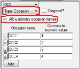
Note that, if Allow arbitrary occasion names is checked, two columns are presented in which arbitrary occasion names (including non-numeric) can be entered in the left column and corresponding numeric values on the right.
The checkbox labeled Diagonal is discussed a little later.
-
Select the Random Effects tab.
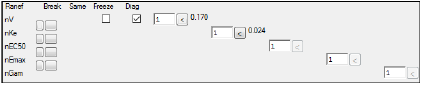
In the upper box are simple random effects, one for each structural parameter that has randomness. The reason there is no checkbox under Same is because there is only one block, and that option only appears between blocks and only if they are the same shape. If Same is checked, it means that the lower block shares the same matrix as the upper block. In this case, the lower block is not displayed because its numbers cannot be edited.
The lower box has the first block of random effects for the occasion covariate effect. There are actually four blocks, one for each value of the occasion covariate, but only the first is shown, because the other three are all the same as the first. Note that there is no button for Break, and no checkbox for Same. That is because the IOV random effect structure is entirely specified by the choices made on the previous tabs, so they cannot be changed here. Also note that, in this case, the omega matrix for these three random effects is a lower-triangle block, not diagonal. It can be made diagonal by checking the Diagonal checkbox previously mentioned on the Covar. Type tab.
It is helpful to see what this does in the generated model text.
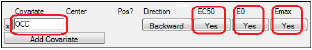
-
OCC is declared to be a covariate:
covariate(OCC)
-
The random effects are declared using the “same” notation:
ranef(block(nE0x0,nEC50x0,nEmaxx0)=c(0.1,0,1,0,0,1)
, same(nE0x1,nEC50x1,nEmaxx1)
, same(nE0x2,nEC50x2,nEmaxx2)
, same(nE0x3,nEC50x3,nEmaxx3)
)
Note that there are four sets of three random effects each. The omega matrix for the first set is shared by the following three.
-
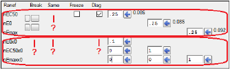
The way these random effects appear in the model is that the value of the OCC covariate selects which random effect is active at any one time, like this:
stparm(EC50=tvEC50*exp(nEC50
+ nEC50x0*(OCC == 1)
+ nEC50x1*(OCC == 2)
+ nEC50x2*(OCC == 3)
+ nEC50x3*(OCC == 4)
))
(There are further statements for each of the structural parameters to be effected.) This differs from a typical categorical covariate effect in which the covariate selects a fixed effect, as opposed to a random effect.
The Fixed Effects tab allows users to enter initial, lower, and upper values for the fixed effects. Every selection made in the Structural tab changes the code for the modified structural parameter. These code changes are displayed in the Model Text tab.
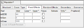
Entering lower and upper values for the fixed effects are optional.
-
In the Initial field, type an initial value for each fixed effect.
-
In the Lower field, type a lower limit value. May be specified by itself or with an upper limit value.
-
In the Upper field, type an upper limit value. May be specified by itself or with a lower limit value.
Only use boundaries if the model converges on a solution that makes no physical sense, such as a negative rate constant or negative volume. If boundaries are entered, the program automatically transforms the parameter to an unbounded space.
For a one-sided bound, an exponential transformation is used. For a two-sided bound, a logistic transformation is used. This transformation is done internally during the optimization phase and the transformed parameter never appears in any results reported to the user. The internal parameter in unbounded space is always transformed back to the original bounded space before results are reported.
Note that, for the QRPEM engine, bounds are ignored. -
Check the Freeze checkbox to fix the parameter estimates to the values entered in the initial, lower, and upper fields.
The Estimate area is blank before a model is executed, but will automatically show parameter estimates after the model is successfully executed. Users can choose to accept these estimates as the new initial estimates. (See “Parameters and parameter mappings” for more information on estimate setup.) -
Click Accept All Fixed+Random to copy all new initial estimates values for all fixed effects, random effects, and the standard deviation.
 The Estimate area only shows the results of the last model run, so when modeling individual subjects, only the estimates of the last subject are displayed.
 -
In the Units field(s), enter the desired unit of measurement for the fixed effect. When executed, the units are applied to the output. If the data has units, the fields are disabled. (See “Units labeling” for more information on handling of units.)
The Random effects tab is only available for population models. Changes made to random effects are reflected in the Model Text tab.
-
Click the Swap random effects
 button multiple times to toggle the positions of the random effects and customize the omega matrix structure.
Random effects in the omega matrix can be swapped as many times as needed. For example, it is possible to move the first fixed effect to the bottom of the list and move the last fixed effect to the top of the list. -
Click the Split or join the random effect blocks
 button, shown under Break, multiple times to toggle splitting or joining the random effects and create multiple omega matrix structures.
The Same checkbox is displayed if the random effect blocks are split more than once, or if splitting the blocks groups together two or more random effects separately from the others. At least two distinct blocks must be created before the Same checkbox can be used, and the blocks must be of the same size. -
Check the Same checkbox if the random effects block is the same as the previous one.
Any selections made to the previous block are reflected in the ones marked as the same. Blocks that are marked as being the same have all their user interface options removed.
Note:When a covariate is declared to be an interoccasion covariate in the UI, the Random Effects tab provides an omega block for a single occasion. Therefore, the Break and Same boxes will not be available for this part of the omega matrix. A textual model would need to be used if a different behavior were desired.
-
Check the Freeze checkbox to freeze the initial omega estimate values at their set values by removing the omega elements from the optimization routine.
The initial estimates are still used in the model, but Phoenix does not try to optimize the estimates and does not offer better estimates after a modeling run. Also, the eta values are different in the output when the initial omega estimate are frozen. -
Use the Diagonal? checkbox to set the interoccasion covariance to a diagonal structure (box is checked, this is the default) or block structure (box is unchecked).
After a model is run, and if the random effects are not frozen, then Phoenix automatically displays new omega estimates. -
Click the Copy omega estimate to initial estimate
 button to copy the new estimate to the initial omega estimate field.
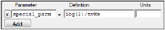
The Secondary tab allows users to add secondary parameters to the model.
-
Click Add to add a secondary parameter.
-
In the Parameter field, type a name for the secondary parameter.
-
In the Definition field, type a definition for the secondary parameter.
•Enter the right side of an equation that uses parameters available in the model.
•The equation must be a function of fixed effects such as tvV and/or covariates. Refer to the “Supported Math Functions” and “Supported Special Functions” for a list functions that are supported.
•Secondary parameters depending on categorical covariate effects do not work for Built-in or Graphical models. The user interface does not accept them. However, they do work for Textual models. For example, if “sex” is a categorical covariate having values 0 and 1, and it modifies column “V,” then there is a fixed effect named “dVdsex1.” This fixed effect is not recognized in the secondary parameter definition; however it will work in a Textual model.
-
In the Units field, enter the units for the parameter, if needed. When executed, the units are applied to the output. If the data has units, the field is disabled.
-
Click the X button to remove a secondary parameter.
Note:Tmax can be defined as a secondary parameter by using the function CalcTMax, e.g.:
secondary(Tmax=CalcTMax(tvA,tvAlpha,tvB,tvBeta,C,Gamma))
If a Tlag variable is included in the dosepoint statement, this postpones the dosing by Tlag, so Tlag should be added into the secondary parameter definition for Tmax, e.g.:
secondary(Tmax=CalcTMax(tvA,tvAlpha,tvB,tvBeta,C,Gamma)+tvTlag)
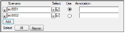
The Scenarios tab is only available for population models. The Scenarios tab lists all covariates effects in the model. If there are no covariate effects in the model, then there is no need to add scenarios.
If the Covariate Search Stepwise or the Covariate Search Shotgun run options are selected in the Run Options tab, then Phoenix automatically creates scenarios during the modeling run, but only if covariate effects are used in the model. The new scenarios are added to the Scenarios tab.
Note:Scenarios are run in the order they are listed on the Scenarios tab.
-
Click Add to add a scenario to append a new scenario,
Or
Insert a new scenario between scenarios by clicking the + button of the preceding scenario. -
Accept the default scenario name or type a new one.
-
Check the Select checkbox to include the scenario(s) in a modeling run.
-
In the Annotation field, type a description of the scenario.
-
Select the Use option button for the scenario to use when the Simple run mode is selected in the Run Options tab.
In Simple run mode, only one scenario can be used during the modeling process. The Use option button determines which scenario is used during a simple run, no matter how many scenarios are selected. -
Click All to select all scenarios.
-
Click None to clear all scenario selections.
-
To run the scenario(s), select the Run Options tab and choose the Scenarios run mode.
