The Phoenix Model Object

Run Options tab

The Run Options tab allows users to determine how Phoenix executes a model. For individual modeling, the jobs are always run locally using the run method Naive-pooled, which cannot be changed. Population modelers have many more run options.

For detailed explanations of Phoenix Model run methods, see “Run modes”.

•Individual modeling run options

•Population modeling run options

•Run Modes

•Simple run mode table options

•Predictive Check Options

•Simulation Options

Individual modeling run options

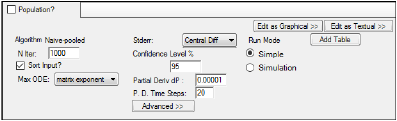
The following options are displayed on the Run Options tab when the Population? checkbox is unchecked.

In the N Iter field, type the maximum number of iterations to use with each modeling run (the default is 1000 and the maximum is 10,000).
Check the Sort Input? checkbox (the default) to sort the input by subject and time values.

If Sort Input? is checked, then the ordering of the subjects in the dataset is not relevant, and all subject IDs are unique. That is, Subject ID 1 refers to subject 1 no matter where Subject ID 1 is listed in the dataset. However, if Sort Input? is not selected, then the ordering of the subjects in the dataset determines whether or not that particular subject ID is treated as new subject. For example, suppose that the ordering of Subject IDs in the dataset are as follows: 1, 2, 3, 1. Phoenix determines that there are four unique profiles, rather than three.
In the Max ODE menu, select one of the ODE (ordinary differential equations) solver methods: matrix exponent, auto-detect, non-stiff, stiff.

For more on ODE methodology, see “Differential equations in NLME”.

Standard errors for the parameters are computed using the Hessian method of parameter uncertainty estimation. The Hessian method evaluates the uncertainty matrix as R-1, where R-1 is the inverse of the second derivative matrix of the -2*Log Likelihood function.

Note:Computing the standard errors for a model can be done as a separate step after model fitting. This allows the user to review the results of the model fitting before spending the time computing standard errors.

For engines other than QRPEM:
– After doing a model fitting, accept all of the final estimates of the fitting.
– Set the number of iterations to zero.
– Rerun with a method selected for the Stderr option.

For QRPEM, use the same steps, but also request around 15 burn-in iterations.

In the Stderr menu, select the method used to compute standard errors.

•none (no standard error calculations are performed)

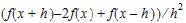
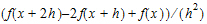
•Central Diff for the second-order derivative of f uses the form:

(1)

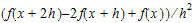
•Forward Diff for the second-order derivative of f uses the form:

(2)

In the Confidence Level % field, enter the confidence interval percentage.
In the Partial Deriv dP field, enter the amount of perturbation to apply to parameters to obtain partial derivatives.
Enter the number of time steps in the P. D. Time Steps field.

Plots of the partial derivatives are spaced at this number of time vales over the whole time line. To get a coarse plot, specify a low number. To get a smoother plot, specify a larger number of steps.

Population modeling run options

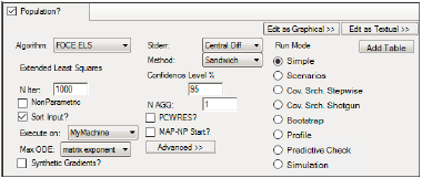
The following options are displayed in the Run Options tab when the Population? checkbox is checked.

Not all run options are applicable for every run method. Some options are made available or unavailable depending on the selected run method. For detailed explanations of Phoenix Model run options, see “Run Modes”.

In the Algorithm menu, select one of seven run methods:

•FOCE L-B (First-Order Conditional Estimation, Lindstrom-Bates)

•FOCE ELS (FOCE Extended Least Squares)

•FO (First Order)

•Laplacian

•Naive pooled

•IT2S-EM (Iterated two-stage expectation-maximization)

•QRPEM (Quasi-Random Parametric Expectation Maximization)

In the N Iter field, type the maximum number of iterations to use with each modeling run (the default is 1000).
Check the NonParametric checkbox to use the NonParametric engine for producing nonparametric results in the output. This option is available for FOCE L-B, FOCE ELS, Laplacian, IT2S-EM, and QRPEM methods.

•If the NonParametric checkbox is selected, then the N NonPar field is made available.

•In the N NonPar field, type the maximum number of iterations of nonparametric computations to complete during the modeling process.

Check the Sort Input? checkbox (the default) to sort the input by subject and time values.

If Sort Input? is selected, then the ordering of the subjects in the dataset is not relevant, and all subject IDs are unique. That is, Subject ID 1 refers to subject 1 no matter where Subject ID 1 is listed in the dataset. However, if Sort Input? is not selected, then the ordering of the subjects in the dataset determines whether or not that particular subject ID is treated as new subject. For example, suppose that the ordering of Subject IDs in the dataset are as follows: 1, 2, 3, 1. Phoenix determines that there are four unique profiles, rather than three.
Select the local or remote machine or grid on which to execute the job from the Execute on menu.

The contents of this menu can be edited, refer to “Compute Grid preferences”.

Note:When a grid is selected, loading the grid can take some time and it may seem that the application has stopped working.

Make sure that you have adequate disk space on the grid for execution of all jobs. A job will fail on the grid if it runs out of disk space.

In the Max ODE menu, select one of the ODE (ordinary differential equations) solver methods. For more on ODE methodology, see “Differential equations in NLME”.
Check the Synthetic Gradients? checkbox to allow synthetic gradients in the model.

When this is selected in population modeling, the engine computes and makes use of analytic gradients with respect to etas. In some cases, with differential equation models, one or more gradient components can be computed by integrating the sensitivity equations along with the original model system using a numerical differential equation solver. For reasonably-sized models, selecting Synthetic Gradients can help speed and accuracy.
In the Stderr menu, select the form of standard error to compute:

•none (no standard error calculations are performed)

•Central Diff, that uses the form:

(3)

•Forward Diff, that uses the form:

(4)

Select the Method of computing the standard errors from the menu:

•Hessian: The Hessian method of parameter uncertainty estimation evaluates the uncertainty matrix as R-1, where R-1 is the inverse of the second derivative matrix of the -2*Log Likelihood function. This is the only method available for individual models.

•Sandwich: Sandwich estimators for standard errors have both advantages and disadvantages relative to estimators based on just the second derivatives (Hessian matrix) and the log likelihood. The main advantage is that, in simple cases, sandwich estimators are robust for covariance model misspecification, but not for mean model misspecification. The main disadvantage is that they can be less efficient than the simpler Hessian-based estimators when the model is correctly specified.

•Fisher Score: The Fisher Score method is fast and robust, but less precise than the Sandwich and Hessian methods.

•Auto-detect: When selected, NLME automatically chooses the standard error calculation method. Specifically, if both Hessian and Fisher score methods are successful, then it uses the Sandwich method. Otherwise, it uses either the Hessian method or the Fisher score method, depending on which method is successful. The user can check the Core Status text output to see which method is used.

In the Confidence Level % field, enter the confidence interval percentage.
In the N AGQ field, enter the maximum number of integration points for the Adaptive Gaussian Quadrature. This field is available for FOCE ELS and Laplacian methods.
In the ISAMPLE field, enter the number of sample points. For each subject, the joint likelihood, the mean, and the covariance integrals will all be evaluated with this number of samples from the designated importance sampling distribution. Increasing this number improves the accuracy of the integrals. This option is available for the QRPEM method.
Check the PCWRES? checkbox to generate the predictive check weighted residuals in the results. This option is available for FOCE L-B, FOCE ELS, FO, Laplacian, and IT2S-EM methods. and is unchecked by default. When checked, then the nrep field becomes available. Enter the number of replicates for predictive check weighted results.

PCWRES is an adaptation of France Mentre’ et al.'s normalized predictive error distribution method. Each observation for each individual is converted into a nominally normal N(0,1) random value. It is similar to WRES and CWRES, but computed with a different covariance matrix. The covariance matrix for PCWRES is computed from simulations using the time points in the data.
Check the MAP-NP Start? checkbox to perform Maximum A Posteriori initial Naive Pooling. This option is available for FOCE L-B, FOCE ELS, FO, Laplacian, QRPEM and IT2S-EM methods. If selected, an Iterations field appears requesting the number of iterations to apply MAP-NP.

This process is designed to improve the initial fixed effect solution with relatively minor computational effort before a main engine starts. It consists of alternating between a Naive pooled engine computation, where the random effects (eta’s) are fixed to a previously computed set of values, and a MAP computation to calculate the optimal MAP eta values for the given fixed effect values that were identified during the Naive Pooled step.

On the first iteration, MAP-NP applies the standard Naive pooled engine with all etas frozen to zero to find the maximum likelihood estimates of all the fixed effects. The fixed effects are then frozen and a MAP computation of the modes of the posterior distribution for the current fixed effects parameters is then performed. This cycle of a Naive pooled followed by MAP computation is performed for the number of requested iterations. Note that, throughout the MAP-NP iteration sequence, the user-specified initial values of an eps and Omega are kept frozen.
Check the FOCEHess? checkbox to use FOCE Hessian. This option is available for Laplacian, Naive pooled and IT2S-EM methods.
Click Advanced to toggle access to advanced run options for population models (only).

All engines have the following Advanced options.

•In the LAGL nDig field, enter the number of significant decimal digits for the LAGL algorithm to use to reach convergence. Used with FOCE ELS and Laplacian Run methods. LAGL, or LaPlacian General Likelihood, is a top level log likelihood optimization that applies to a log likelihood approximation summed over all subjects.

•In the SE Step field, enter the standard error numerical differentiation step size. SE Step is the relative step size to use for computing numerical second derivatives of the overall log likelihood function for model parameters when computing standard errors. This value affects all Run methods except IT2S-EM, which does not compute standard errors.

•In the BLUP nDig field, enter the number of significant decimal digits for the BLUP estimation to use to reach convergence. Used with all run methods except Naive pooled. BLUP, or Best Linear Unbiased Predictor, is an inner optimization that is done for a local log likelihood for each subject. BLUP optimization is done many times over during a modeling run.

•In the Modlinz Step field, enter the model linearization numerical differentiation step size. Modlinz Step is the step size used for numerical differentiation when linearizing the model function in the FOCE approximation. This option is used by the FOCE ELS and FOCE L-B Run methods, the IT2S-EM method when applied to models with Gaussian observations, and the Laplacian method when the FOCEhess option is selected and the model has Gaussian observations.

•In the ODE Rel. Tol. field, enter the relative tolerance value for the Max ODE.

•In the ODE Abs. Tol. field, enter the absolute tolerance value for the Max ODE.

•In the ODE max step field, enter the maximum number of steps for the Max ODE.

The following are additional advanced options available only for the QRPEM method.

Check the MAP Assist checkbox to perform a maximization of the joint log likelihood before each evaluation of the underlying integrals in order to find the mode. The importance sampling distribution is centered at this mode value. (If MAP Assist is not selected, the mode finding optimization is only done on the first iteration and subsequent iterations use the mean of the conditional distribution as found on the previous iteration.) If the MAP Assist checkbox is checked, enter the periodicity for MAP assist in the period field. (For example, a value of two specifies that MAP assist should be used every other iteration.)
Select the importance sampling distribution type from the Imp Samp Type pull-down menu.

•normal: Multivariate normal (MVN)

•double-exponential: Multivariate Laplace (MVL). The decay rate is exponential in the negative of the sum of absolute values of the sample components. The distribution is not spherically symmetric, but concentrated along the axes defined by the eigenvectors of the covariance matrix. MVL is much faster to compute than MVT.

•direct: Direct sampling.

•T: Multivariate t (MVT). The MVT decay rate is governed by the degrees of freedom: lower values correspond to slower decay and fatter tails. Enter the number of degrees of freedom in the Imp Samp DOF field. A value between four and 10 is recommended, although any value between three and 30 is valid.

•mixture-2: Two-component defensive mixture. (See T. Hesterberg, “Weighted average importance sampling and defensive mixture distributions,” Tech. report no. 148, Division of Biostatistics, Stanford University, 1991). Both components are Gaussian, have equal mixture weights of 0.5, and are centered at the previous iteration estimate of the posterior mean. both components have a variance covariance matrix, which is a scaled version of the estimated posterior variance covariance matrix from the previous iteration. One component uses a scale factor of 1.0, while the other uses a scale factor determined by the acceptance ratio.

•mixture-3: Three-component defensive mixture. Similar to the two-component case, but with equal mixture weights of 1/3 and scale factors of 1, 2, and the factor determined by the acceptance ratio.

Check the MCPEM checkbox to use Monte-Carlo sampling instead of Quasi-Random. Although the default is recommended, using Monte-Carlo sampling may be necessary if the most direct comparison possible with other MCPEM algorithms is desired.
Check the Run all checkbox to execute all requested iterations, ignoring the convergence criteria.
In the # SIR Samp field, enter the number of samples per subject used in the Sampling Importance Re-Sampling algorithm to determine the number of SIR samples taken from the empirical discrete distribution that approximates the target conditional distribution.

The # SIR Samp from each subject are merged to form the basis for a log-likelihood optimization that allows fixed effects that are not paired with random effects to be estimated. The # SIR Samp is usually far smaller than the number that would be used if the SIR algorithm were not used.

The default of 10 is usually adequate, unless the number of subjects is extremely small. If necessary, # SIR Samp can be increased up to a maximum of ISAMPLE.
In the # burn-in Iters field, type the number of QRPEM burn-in iterations to perform at startup to adjust certain internal parameters. During a burn-in iteration, importance sampling is performed and the three main integrals are evaluated, but no changes are made to the parameters to be estimated or the likelihood. The default is zero, in which case the QRPEM algorithm starts normally. Typical values, other than zero, are 10 to 15.
Check the Frozen omega burn-in checkbox to freeze the omega but not theta for the number of iterations entered in the # burn-in Iters field. If this checkbox is not checked, then both omega and theta are frozen during the burn-in.
Check the Use previous posteriors checkbox to start the model up from the posteriors and eta-means saved from a previous run. Checking this box allows the QRPEM engine to be restarted from a previous run using the final posteriors from that run as initial posteriors in the restart, thus allowing the run to resume from exactly where it left off. To do this, press Accept All Fixed+Random in the Parameters tab to accept the final parameter estimates from the first run as initial parameter estimates for the new run, then run QRPEM with the Use previous posteriors box checked.
In the Acceptance ratio field, enter a decimal value for the acceptance ratio (default is 0.4). As this value is reduced below 0.4, the importance sampling distribution becomes broader relative to the conditional density.

Note:ISAMPLE, Imp Samp Type, and Acceptance ratio can all be used to increase or decrease the coverage of the tails of the target conditional distribution by the importance sampling distribution.

Select the Quasi-Random scrambling method to use from the Scramble menu: none, Owen, or TF (Tezuka-Faur).

Run Modes

Only the Simple and Simulation run modes are available for individual models. (Refer to “Run Modes” for more details about the following modes.)

Simple: (The default mode.) Only estimate parameters. See “Simple run mode table options”.
Scenarios: Use if scenarios are defined for a model.
Cov. Srch. Stepwise: Add scenarios to a model as it is being run. Use the Criterion menu to select information criterion to use. In the Add P-Value and Remove P-Value fields, enter the threshold values at which to add or remove a covariate effect.
Cov. Srch. Shotgun: Add scenarios to a model as it is being run. Use the Criterion menu to select information criterion to use.

The best scenario found after using Stepwise or Shotgun is automatically selected in the Scenarios tab. The selected scenario is used for any subsequent Simple runs. An example of a selected scenario that was created after using the covariate search stepwise mode is shown below.

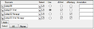
Covariate Stepwise and Shotgun searches only generate the Overall worksheet as an output worksheet. To generate the full results, change the Run Mode to Scenarios in the Run Options tab and re-execute. Since the best scenario is selected automatically after the covariate search, it will be used during the Scenarios run.

Bootstrap: In the Seed field, enter an initial seed value for the random sampling. Each subsequent bootstrap sample will use a different seed. Check the Keep? checkbox to use the same starting seed for the next run. Enter the number of samples for the Bootstrap mode in the # samples field. If covariates are specified, then users can select up to three optional covariate to use to stratify the bootstrapping process. In the max tries field, enter the maximum number of Bootstrap iterations to perform.
Profile: Perform likelihood profiling. All fixed effects in the model are listed. Check the Profiling checkbox beside each fixed effect to include it in the profile and enter profile deltas, separated by commas, in the Perturbations field. Click Perturbations multiple times to toggle between Perturbations (%) (values are entered as percentages) and Perturbations (Amt) (values are entered as simple amounts).
Predictive Check: In the Seed field, enter an initial seed value for the random sampling. Each subsequent sample will use a different seed. Check the Keep? checkbox to use the same starting seed for the next run. Other predictive check options are located in several tabs in the Predictive Check Options area. For option descriptions, see “Predictive Check Options”.

For details about predictive check usage, see “Predictive Check run mode”.
Simulation: A model is only evaluated in a simulation run, not fitted. All engines will bypass the fitting if Simulation is selected (for Naive pooled, the variance inflation factor computation is done). For option descriptions, see “Simulation Options”.

Simple run mode table options

If the Simple run mode is selected, users can add extra tables to the output. For example, users can specify an output table whose rows represent instances where particular covariates are set, or particular dosepoints receive a dose, or particular observables are observed.

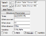
Click Add Table to include an extra results tables that contain user-specified output.

Several options are made available. Users can enter their own values in the new fields to create custom table output that is sorted on a per profile basis.

Check the checkbox after the table name to view/modify the table settings for that table.
Click the X button to delete the corresponding table.
Enter a brief description of the custom output table in the field.

All model variables, including stparms, fixefs, secondary, and freeform assigned variables, can be added as output in the table.

Click Structural Parameter to add the parameters defined in the Structural tab to the Variables field.
In the Times field, enter sampling times to include in the tables. For example, 0.1, 1, 5, 12. A row is generated in the table for each time.

Additionally, a sequence statement like “seq(0,20,1)” can be used to convey that the times to output in the table should be from zero to 20 by 1 unit of time (e.g., 0, 1, 2, 3, …, 20). The first argument in the seq statement is the starting time point, the second argument is the last time point, and the third argument indicates the time increments.
In the When covr set field, enter the covariates used, if any. For example, age, weight, gender. A row is generated in the table at any time at which the specified covariate value is set (not missing).
In the When dose field, enter the dose point to include in the table. For example, Aa or A1. A row is generated in the table at any time at which a dose is administered to the specified compartment, if dosing data is provided in the input source or a dosing worksheet.
In the When observe field, enter any observations to include in the table. For example, CObs or EObs. A row is generated in the table at any time at which the specified observation is made.
In the Variables field, enter any additional variables not applicable in the other fields. For example, Cl or Tlag. A column is added to the table for each variable specified in the list.

For example, to capture concentration and a secondary parameter called C2 at each observation of concentration and at time 7.5 enter 7.5 in the Times field, Cobs in the When Observe field, and C and C2 in the Variables field.
Check the boxes for TAD, IRES, Weight, and IWRES, to include these values in a Table. For IRES, Weight, and IWRES, specify an observation for the When observe option to make the checkboxes become available.
The variable names are case sensitive. If the table is not produced as expected, check the case of the variable names in the table specification.

Predictive Check Options

•Main tab

•Observation tabs

Main tab

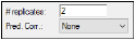
In the # replicates field, enter the desired number of replicates. This is the number of datasets that are sampled to perform the population prediction. The maximum number of replicates allowed is 10,000. If the user enters a larger number, only 10,000 will be generated. The value entered applies to all dependent variables.
Optionally use the Pred. Corr. (Prediction Correction) pull-down menu to specify the type of correction to use to calculate a prediction-corrected observation. This option applies to all dependent variables except in time-to-event cases, where this option is ignored. (See “Prediction and Prediction Variance Corrections” for calculation details.)

•None: do not apply a correction

•Proportional: use the proportional rule. Choosing this option displays the Pred. Variance Corr. option. If this checkbox is turned on, a prediction-variability corrected observation will be calculated and used in the plots.

•Additive. use the additive rule. Choosing this option displays the Pred. Variance Corr. option. If this checkbox is turned on, a prediction-variability corrected observation will be calculated and used in the plots.

Note:If the observations do not typically have a lower bound of zero, the Additive option may be more appropriate.

Observation tabs

For each continuous observation in the model, a separate tab is made available.

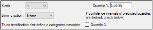
Specify the variable to use for the X axis in the predictive check plots from the X axis pull-down menu.

•t is time (the default)

•TAD is time after dose

•PRED is population (zero-eta) prediction

•other... displays a field to type in the name of any other variable in the model

Prediction intervals, or the quantiles of the predictive check simulation, might not be very smooth if there are a lot of time deviations in the dataset. The predictive check has the option whether or not to bin the independent variable.

For continuous observations, select the binning method to use from the Binning option pull-down menu. Different binning methods can be specified for different dependent variables.

•None: Every unique X-axis value is treated as its own bin (the default method)

•K-means: Observations are initially grouped into bins according to their sequence order within each subject. Then the K-means algorithm rearranges the contents of the bins so every observation is in the bin that has the nearest mean X value or “center of gravity.” Starting with an initial set of bins containing observations (with a mean X value of these observations), the K-means algorithm:

1) transfers each observation to the bin with the closest mean to the observation, and
2) recalculates the mean of each bin. This is repeated until no further observations change bins. Bins that lose all their observations are deleted.

Note that the algorithm is sensitive to the initial set of bins.

•Explicit centers: Specify a series of X values to use as the center values for each bin. Observations are placed into the nearest bin.

•Explicit boundaries: Specify a list of X value boundaries between the bins. Observations are placed in the nearest bin. The center value of each bin is taken as the average X value of the observations in the bin.

In the case of Explicit centers and Explicit boundaries, the numerical values, separated by commas, are automatically sorted into ascending order and duplicates are eliminated. In all cases, bins having no observations are eliminated.

In the Stratify menu, select a defined categorical covariate.

This option is available if a categorical covariate is defined for stratifying the Predictive Check simulation. Defined categorical covariates can be used to stratify the modeling simulation. Up to three levels of stratification are available and the same stratas are applied for all dependent variables.
Check the BQL checkbox and select an option from the menu to specify the way BQL data is handled. (Only available if the BQL? checkbox in the Structure tab is checked or the argument is included in textual mode).

•Select Treat BQL as LLOQ to replace BQL data less than the LLOQ value with the LLOQ value in Observations and related worksheets.

•Select BQL Fraction from the menu to have the amount of BQL data checked and its fraction compared with the quantile level. If the fraction of BQL data is more than the defined quantile, the corresponding observed data are not shown in the VPC plot or in PredCheck_ObsQ_SimQCI/ PredCheck_SimQ and Pop PredCheck ObsQ_SimQCI/ Pop PredCheck SimQ.worksheets.

For a categorical observation, the Time-to-event checkbox becomes available in cases of event, count, LL, or multi-statement. When checked, the time field shows the same syntax as in the simulation tab and additional worksheets are generated (Simulation table 01, Simulation table 02,..., Predcheck_TTE).

Note that, in the case of time-to-event simulations, only the first event is used; subsequent events are ignored.
For continuous data, in the Quantile % field, accept the default quantiles or enter new ones.

If more than one quantile is used, they must be separated by a comma. For example, 10,50,90. The default quantiles are 5, 50, and 95. Different quantiles can be specified for different dependent variables.
Check the Quantile checkbox to include predicted quantiles confidence intervals in the predictive check output. If this option is not checked for a dependent variable, then the associated plot will be the same as the Pop PredCheck_SimQ plot.

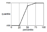
The quantiles are the summary statistic measures provided by the predictive check. There are multiple ways to calculate quantiles, given percentiles and a data set. NLME uses the same method as SPSS, and R’s quantile function with type=6. The following diagram illustrates the quantile function in the case of a dataset containing three numbers. The numbers are sorted in ascending order. If there are N numbers, there are N+1 intervals. Percentiles (expressed as fraction F) falling below 1/(N+1) or above N/(N+1) have a quantile equal to the minimum or maximum, respectively. Otherwise the quantile is found by linear interpolation.

Users can optionally select to calculate confidence intervals for the predicted intervals, or predictive check quantiles. Since each simulated replicate is like the original dataset, first the quantiles are obtained at each stratum-bin-time for each replicate. For each stratum-bin-observed quantile, users get a cloud, one for each replicate. Then quantiles of the quantiles are calculated by stratum-bin-time over all replicates corresponding to a confidence interval of the simulated quantiles.

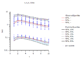
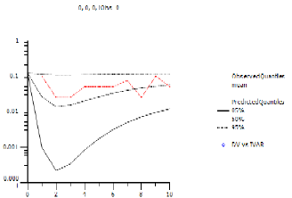
With predictive check, there is one level of simulated quantiles of observations (e.g., the values entered in the Quantile % field). During simulation, the model is purposely disturbed so that the predicted values of the observations fall in a range. The intent is to determine if the range includes the actual observations that came in on the original data. The Pop PredCheck ObsQ_SimQ plot shows the simulated quantiles:

The blue dots are the actual original observations. The red lines are 5%, 50%, and 95% quantiles from the actual original observations. The black lines are the 5%, 50%, and 95% quantiles from the simulated observations. The example plot above shows a good match between them.

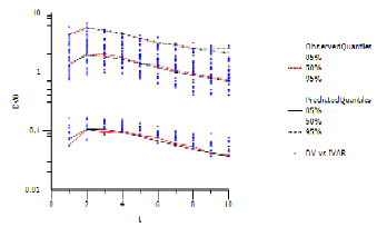
Sometimes the user wants to determine the confidence level of the simulated quantiles. To see how much the simulated quantiles are themselves variable, check the Quantile checkbox. This provides an additional plot of confidence intervals of the simulated quantiles (Pop PredCheck ObsQ_SimQCI plot).

In place of each simulated quantile black line, there are two black lines, representing the 10% and 90% confidence intervals of that quantile. The shading aids in visualizing the variation. Notice how the red lines fall inside the black lines (i.e., within the shaded area), which is a positive result.

If there are additional observations from a questionnaire involved, the observation cannot be predicted, only the likelihood of each possible answer can be observed or predicted. If, for example, there are four answers to the questionnaire: 0, 1, 2, 3, then there will be four observations or predictions. The following image shows the Pop PredCheck ObsQ_SimQ plot for observation 0.

The red line is the actual fraction of observations that were 0. The black lines are the 5%, 50%, and 95% quantiles of the predicted probability of seeing 0. Note that the red line falls between the black line most of the time.

Simulation Options

A Phoenix Model can also perform a Monte Carlo population PK/PD simulation for population models when the Simulation run mode is selected. Simulations can be performed with built-in, graphical, or textual models. Two separate simulations are performed automatically if a table is requested, one simulation for the predictive check, and another simulation for each table. A simulation table contains only a time series and a set of variables. If one of the variables is a prediction, like C, then its observed variable, like CObs, is also included and simulated with observational error.

The following options are specific to the type of simulation model: Individual or Population.

For Individual models:

•Specify the number of simulated data points to generate in the # points field. The maximum number of simulation points allowed is 1,000. The value entered applies to all dependent variables.

•Use the Max X Range field to specify the maximum time or independent variable value used in the simulation.

•In the Y variables field, specify the desired output variable(s) to capture from the model. The captured variable(s) is displayed, in # points equal time/X increments, in the simulation worksheet.

•Check the Sim at observations? checkbox to have the simulation occur at the times that observations happen as well as at the given time points.

•Add other simulation tables using the other tools in the same manner as under Predictive Check.

For Population models:

•Specify the number of simulated replicates to generated in the # replicates field. The maximum number of replicates allowed is 10,000.

•If desired, designate a directory for the result files in the Copy result files to directory field or use the button. If a directory is defined, a csv file with simulation results for all replicates will be placed there.

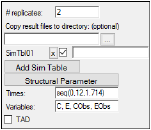
Click Add Sim Table to add a simulation table.

Multiple simulation tables can be added. Users can enter unique names for each table in the field next to the checkbox. These names are NOT used in the simulation results. For every simulation table added here, there is a results worksheet generated called Simulation Table 01 (up to 5).
Enter a time sequence in the Times field using the following format: seq(<start time>,<end time>,<time increment>).

For example, seq(0,20,1) specifies that a sequence of times from zero to 20 incremented by 1 time unit (0, 1, 2, 3, …, 20) is created.
Enter simulation variables in the Variables field. Variables must be separated by a comma (,).

For example, entering C, E, CObs, EObs specifies that C and E are simulated individual predicted values (simulated IPREDs), and that CObs and EObs are simulated observations.
Click Structural Parameter to add all structural parameters in the model to the Variables field.
Check the TAD checkbox to add a time after dose column to the simulation table. The TAD column is added to the Rawsimtbl01.csv results file.
Check the checkbox beside each table to view that table’s options.
Click the X button to remove a simulation table.

A worksheet and a simulation file are created in the results: PredCheckAll and Rawsimtbl01.csv. The simulation file is created externally because depending on the number of replicates it can be very large and affect performance. The PredCheckAll worksheet contains the predictive check simulated data points and Rawsimtbl01.csv contains the simulated data. All other results correspond to the model fit because Phoenix fits the model before performing simulations.