Run modes available for the Phoenix Model include:
The Simple run option estimates the parameters for the specified model with the selected options and engine method. If no sort keys are specified, then the Simple run is automatically parallelized using MPI. The Simple option is available for Population and Individual models and allows specifying additional optional output tables. See “Simple run mode table options”.
With the Simple mode and the Table option, users can also simulate the effect of adding additional doses. For example, there could be a column such as ADDL (additional) in the input dataset that can indicate the number of additional doses to add following the observed data. In the Input Options tab, select the ADDL checkbox and click Add and enter values for the dosing regimen to be simulated.
For example, to simulate an additional number of infusions of 50 dose units infused at a rate of 100 every 72 time units, the following selections must be made:
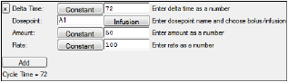
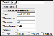
In the Run Options tab, the number of iterations, N Iter, should be set to zero so that the estimates are fixed. The Simple mode table can be specified to output the times desired to see simulated concentrations. In the screen shot below the request is to output times from zero to 600 in increments of 0.5. Note that requesting the variable “C” indicates that predicted concentration values (C) should be recorded at the times requested and in addition when doses are added to the amount in the central compartment (A1), and when concentrations are observed (CObs).
The Scenarios run mode option is only available for Population Phoenix Models and it requires that scenarios be defined in the Scenarios tab, which is located in the Parameters tab. Scenarios allow users to investigate different combinations of covariate effects on the same structural model. The Scenarios mode is similar to doing a simple run on several models where their base structural model is the same but the covariate effects are different. A Scenarios run is automatically parallelized using MPI. The number of scenarios as the number of replicates (if sort keys are specified, then the number of replicates is computed by multiplying the total number of scenarios by the total number of unique sort keys).
Covariate Search Stepwise run mode
The Cov. Srch. Stepwise (stepwise covariate search) run mode is only available for Population Phoenix Models. Covariates and covariate effects must be specified. This run mode performs an automatically parallelized stepwise forward or backward addition or deletion of covariates effects by adding one at a time to determine if they make a sufficient threshold improvement based on the specified criterion options. (Note that, during the first step, the baseline model is combined with the replicates for the first addition step in order to avoid running the base model alone as the first step.)
There are three options for this mode: the criterion on what to base the stepwise approach (-2LL, AIC, or BIC), the threshold for improvement in the criterion in order to add a covariate effect, and the threshold to remove a covariate effect.
If the -2LL criterion is chosen, instead of providing threshold values for adding and removing effects, the user provides p-values, such as 0.01 and 0.001. These p-values are used, in conjunction with the degrees of freedom for the particular effect, to determine the thresholds using the inverse cumulative distribution function of the chi-square distribution. The degrees of freedom is the number of fixed effects active under the actual current selection of covariate effects. Normally, this is the base set of fixed effects, plus one for each enabled covariate effect. However, if the covariate effect is for a categorical covariate having N categories (N > 1) the number of fixed effects (and thus degrees of freedom) for that covariate effect is N-1.
The stepwise covariate search method used is the forward addition, backwards elimination where the structural model is used as a baseline and the covariate model is made increasingly complex. After each model estimation, the covariates are evaluated to see which one has the greatest improvement in the goodness-of-fit statistic selected (-2LL, AIC, or BIC) greater than the user-specified threshold. That covariate is added to the regression model for the structural parameter and the model is estimated. This process is repeated until all significant effects are accounted for. Then the process works in reverse to eliminate covariates on parameters whose removal produces the smallest reduction in goodness-of-fit less than the user-specified threshold.This process can find a good set of covariate effects more quickly than the shotgun mode.
The stepwise covariate search option creates a list of models, called scenarios, that are listed in the Scenarios tab. The best scenario based on the criterion (-2LL, AIC, or BIC) is selected in the Scenarios tab. All the scenarios evaluated are presented in the results.
How to force some covariates to be part of the model while others are evaluated via the stepwise covariate search
In some Population PK modeling studies, it may be necessary to “force” some covariates to be part of the base model (e.g., Cl=tvCl*(Wt/70)^0.75). However, when it comes to stepwise searching, the rest of the covariates (e.g., age, sex, etc.) need to be tested. This can be accomplished through the text model.
-
In the Run Options tab, click Edit as Text.
-
Look for lines such as:
fixef(dVdwgt(enable=c(0))=c(, 0.949657, ))
fixef(dKedGender1(enable=c(1))=c(, 0.0586368, ))
-
Remove them as desired by deleting or commenting out the enable clause as shown below:
fixef(dVdwgt/*(enable=c(0))*/=c(, 0.949657, ))
fixef(dKedGender1(enable=c(1))=c(, 0.0586368, ))
The covariate search will ignore the covariate that was commented out (or deleted).
Another way to comment out the enable clause is as follows:
/* (enable=c(0)) /**/
The /*...*/ comments are non-nesting, so both of these opening and closing character sets would have to be removed in order to comment the clause back in. Using the /*.../**/ characters makes it easier to comment the clause back in:
(enable=c(0)) /**/
Covariate Search Shotgun run mode
The Cov. Srch. Shotgun (shotgun covariate search) run mode option is only available for Population Phoenix Models. Covariates and covariate effects must be specified. This run mode performs an automatically parallelized shotgun search to evaluate all the possible scenarios and selects the best one out of 2^(number of effects). Each possible effect that is added has the effect of doubling the number of scenarios. It creates a list of evaluated scenarios in the Scenarios Tab. The best scenario based on the criterion (-2LL, AIC, or BIC) is selected in the Scenarios tab. All scenario results are listed in the Results tab.
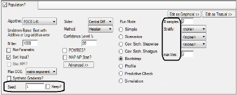
The Bootstrap run mode is only available for Population Phoenix Models. Bootstrap is a diagnostic tool to better understand the precision of estimates. The assumption is that the observations are independent between subjects. Bootstrap consists of running a series of model fits, each time using a random sampling, with replacement, from the original set of individuals. Prior to performing bootstrap Phoenix runs a simple fit to the model and then takes the final estimates of the simple run as initial estimates for all the bootstrap runs. The first run is automatically parallelized using MPI and the number of bootstrap replicates as provided by the user.
For example, if a user has 100 subjects in the original study data, then the created datasets, or resamples, will also contain 100 subjects per each bootstrap run, with some subjects replicated more than once. Several bootstrap samples can be created and all of the samples are individually fitted to the original model in order to obtain a new set of estimated parameters for each sample. After all the samples have been fitted the bootstrapped estimates are summarized. The output should contain the Simple run output and the Bootstrap output.
Bootstrap has four options: the number of samples to create (# samples), the optional stratification of the samples (Stratify), the maximum number of retries (max tries), and the seed number (Seed).
The number of samples requested can be a number from two to infinity, however, very large numbers, such as one million or higher, are discouraged because of memory limitations. The option to stratify a sample by a particular categorical covariate, such as sex, ensures that each unique value that is available for the selected stratification variable will be sampled equally for each Bootstrap run. (In cases where reset blocks are involved, only the first values of covariates in the first reset block are used.)
For example, if a user has 100 subjects that are 50% male and 50% female, then each resampled dataset will have 50 males and 50 females. A maximum of three stratifications can be selected, and the order of the selected stratified variables specifies a nesting structure.
The third option is the maximum number of tries, which accepts numbers from 2 to 99. If a sample fails to converge, it is re-tried as many times as indicated with different random seeds, in an effort to get a full set of samples evaluated. The Seed option is in the Run Options tab, and it is used as an initial seed value for the random sampling. Each subsequent bootstrap sample will use a different seed. Phoenix adds 100 to the starting seed. If the Keep? option is selected then the same starting seed will be used for the next run. Otherwise, Phoenix assigns a random seed and bootstrap results might vary if they are executed twice. The Keep? option only prevents a new seed from being created before the next run.
If scenarios are defined in the Scenarios tab, either by using the covariate search methods or by manually creating them, then the scenario selected by the Use option button in the Scenarios tab is the one used for the Bootstrap procedure.
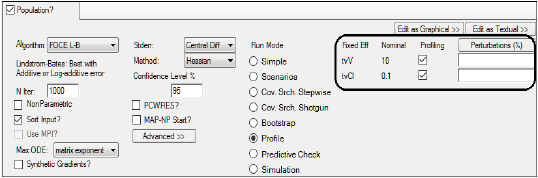
The Profile run mode is only available for Population Phoenix Models. This option performs likelihood profiling to help users understand the sensitivity of the fixed effect parameter estimates on the likelihood. This approach perturbs by an indicated amount or percentage one of the selected fixed effects and fixes, or freezes, it while letting the other model parameters vary. On each perturbation the model is fitted and its results are presented. The user can select the fixed effect(s) to investigate and then enter an amount or percentage value by which to perturb the parameter estimate.
If more than one parameter is selected, the profiling is done as many times as parameters are selected. Each parameter is perturbed by the indicated absolute amount or by a percentage of their estimate, and Phoenix will also display the original parameter estimate without perturbation. If a model is very sensitive to a specific parameter, perturbing that parameter by a small amount will show a large effect on the likelihood.
For example, if the initial estimate of tvV is 10 and a user enters the perturbation values as “–1, 1, 3", then the model is run four times with tvV frozen at 9, 10, 11, and 13. If the initial estimate of tvV is 10 and the perturbation percents are “–10,10”, then the models are run with tvV frozen at 9, 10 and 11. A perturbation of zero is the default value and doesn't need to be entered.
The user selects fixed effects parameters for profiling by placing a selecting the profiling column for the desired parameter. A field is displayed that allows users to enter numeric values separated by a comma (–10, 10). In the Run Options tab, users can switch between perturbations entered by amount or by percentage.
Simulation is useful for situations where modelers have PK/PD parameter estimates from prior modeling and want to explore the potential impact of modifying certain conditions, such as dosing regimens, without having to collect more data. Simulations are based on the structural model and its parameter estimates.
In a Phoenix model, when the run mode in the Run Options tab is set to Simulation, Phoenix performs a PK/PD simulation according to the model settings and PK/PD parameters provided in the user interface. Simulation can be performed with built-in, graphical, or textual models.
Users must enter PK/PD parameter values in the Parameters > Fixed Effects sub-tab. Final estimates created by a previous modeling run can be used as initial estimates. Users can also enter initial estimates in the Fixed Effects tab.
If the input dataset contains multiple subjects, the simulated data will be the same for all subjects unless a parameter values worksheet is mapped to the Parameters panel or the Use Internal Worksheet checkbox is selected in the Parameters panel and values are entered for each subject. Manually entered parameter names must exactly match the names defined in the model. They are also case sensitive (tvKa, for example).
In the Run Options tab, users can specify the number of data points/replicates to be simulated, maximum X (independent variable) range, and the Y (dependent) variable(s) to be simulated. For example, entering 100 in the # points/replicates field, 20 in the Max X Range field, and C, E in the Y variable(s) field simulates a PK/PD model that has 100 data points for C (concentration) and E (effect) between time zero and time 20. Users can also choose to simulate data points at observation times in the dataset.
The Simulation run mode creates a Simulation worksheet containing the simulated data points and an Ind Simulation graph containing simulated data.
The Predictive Check run mode is available for the Phoenix Population Model. When the Predictive Check run option is selected, the model is first fit with 0 iterations (regardless of N Iter in the user interface) in order to generate the data needed to fill the standard results (such as Residuals, Theta, etc.).
To run Predictive Check on the final estimates from a model fitting (Simple run mode), users should accept all final Fixed and Random estimates as the initial estimates for the Predictive Check.
Predictive check is based on the resulting model fit estimates of theta, sigma, and omega. It also uses the estimates of eta(s) for each subject. Each simulation replicate generates a dataset just like the original dataset, except that for each observation there is a simulated observation and replicate 0 will have double the number of observations as other replicates, since it contains both the PRED and the simulated values. Both eta (individual variation) and epsilon (observation error) are sampled and used to create a population prediction. Predictive Check provides a series of summary statistics (quantiles) of the simulated data to compare with the observed data.
Predictive Check run mode provides the option to enter an initial seed value for the random simulation instead of using a random seed. This option is located in the Run Options tab. Each replicate uses a different seed by adding 100 to the starting seed. If the Keep option is checked, then the same starting seed is used for the next run. Otherwise, Phoenix assigns a random seed and predictive check results will vary if the model is run again. The Keep option only prevents a new seed from being created before the next run. The number in the Seed field is retained from the last run.
For an example of a Predictive Check modeling run using a PK/PD model, see the Phoenix NLME User’s Guide Examples chapter. The Predictive Check options are described in “Run modes”.
Note:If the input dataset contains multiple subjects, the simulated data will be the same for all subjects unless a parameter values worksheet is mapped to the Parameters panel or initial parameter values are entered in the Fixed Effects tab.
