Simulation is useful for situations where modelers have PK/PD parameter estimates from prior modeling and want to explore the potential impact of modifying certain conditions, such as dosing regimens, without having to collect more data. Simulations are based on the structural model and its parameter values.
During a Simulation run, a PK/PD simulation is performed according to the model settings and PK/PD parameters provided. All engines bypass fitting if Simulation is selected (for Naive pooled, the variance inflation factor computation is done). Simulation can be performed with built-in, graphical, or textual models.
For built-in and graphical models, users must enter PK/PD parameter values in the Parameters window. Final estimates created by a previous modeling run can be used as initial estimates.
A Monte Carlo population PK/PD simulation is performed based on the values provided for Theta, Omega, and sigma. If a table is requested, two separate simulations are performed automatically, one simulation for the predictive check and another simulation for each table.
-
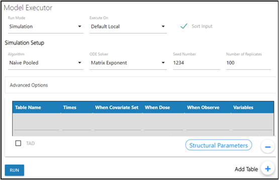
In the Model Executor window, select the Simulation from the Run Mode pulldown.
-
Select the local or remote machine or grid on which to execute the job from the Execute On menu.
The contents of this menu can be modified using preference settings, refer to the “NLME Settings” section in the Pirana user documentation. -
Check the Sort Input checkbox to sort the input by subject and time values.
Refer to the description in the Simple run mode section for more details.
For population models:
Except for the following, descriptions for the Simulation Setup options and Advanced Options can be found in the Simple run mode’s “Estimation” and “Advanced Options” sections.
-
Enter the Seed Number to use as an initial seed value for the random sampling.
-
Specify the number of simulated replicates to be generated in the Number of Replicates field. The maximum number of replicates allowed is 10,000.
-
Click Add Table + to add a simulation table.
For every simulation table added here, there is a results worksheet generated. The options available for a simulation table are described in the Simple run mode “Table” section, except for the following options:
–For Keep source structure, if checked, keeps the number of rows outputted in the table for each simulation replicate the same as the number of rows in the input datasets.
–For the Variables column, the user can enter any variables (separated by a comma) used in the model.
–Click Structural Parameters below the table to add the parameters defined in the model stparm statement to the Variables field.
For individual models:
-
Enter the Number of points to generate for the dependent variables. The maximum number of simulation points allowed is 1,000.
-
Edit the Maximum X range for the maximum independent variable value used in the simulation.
-
Specify model Y variables to be outputted.
-
Check the Sim at observations box to have the simulation occur at the times that observations happen as well as at the given time points.
-
Click Add Table to add a simulation table.
For every simulation table added here, there is a results worksheet generated. The options available for a simulation table are described in the Simple run mode “Table” section, except for the following options:
–For Keep source structure, if checked, keeps the number of rows outputted in the table for each simulation replicate the same as the number of rows in the input datasets.
–For the Variables column, the user can enter any variables (separated by a comma) used in the model.
–Click Structural Parameters below the table to add the parameters defined in the model stparm statement to the Variables field.
