Advanced Options

The following options are available when doing Population modeling. For Individual modeling, only the three ODE options are available.

The advanced options available when QRPEM is selected as the Algorithm are discussed in the “Advanced Options for QRPEM only” section.

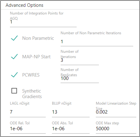
Enter the maximum Number of Integration Points for AGQ in the field.
Available for FOCE ELS and Laplacian methods.
Check the Non Parametric box to use the NonParametric engine for producing nonparametric results in the output.
Available for FOCE L-B, FOCE ELS, Laplacian, IT2S-EM, and QRPEM methods.

If checked, enter the Number of Non Parametric Iterations to complete during the modeling process in the field.
Check the MAP-NP Start box to perform Maximum A Posteriori initial Naive Pooling.
Available for FOCE L-B, FOCE ELS, FO, Laplacian, QRPEM and IT2S-EM methods.

If checked, enter the Number of Iterations to apply MAP-NP in the field.

This process is designed to improve the initial fixed effect solution with relatively minor computational effort before a main engine starts. It consists of alternating between a Naive pooled engine computation, where the random effects (etas) are fixed to a previously computed set of values, and a MAP computation to calculate the optimal MAP eta values for the given fixed effect values that were identified during the Naive Pooled step.

On the first iteration, MAP-NP applies the standard Naive pooled engine with all etas frozen to zero to find the maximum likelihood estimates of all the fixed effects. The fixed effects are then frozen and a MAP computation of the modes of the posterior distribution for the current fixed effects parameters is then performed. This cycle of a Naive pooled followed by MAP computation is performed for the number of requested iterations. Note that, throughout the MAP-NP iteration sequence, the user-specified initial values of an eps and Omega are kept frozen.
Check the PCWRES box to generate the predictive check weighted residuals in the results.
Available for FOCE L-B, FOCE ELS, FO, Laplacian, and IT2S-EM methods.

When checked, enter the Number of Replicates to use for the predictive check weighted results.

PCWRES is an adaptation of France Mentre’ et al.'s normalized predictive error distribution method. Each observation for each individual is converted into a nominally normal N(0,1) random value. It is similar to WRES and CWRES, but computed with a different covariance matrix. The covariance matrix for PCWRES is computed from simulations using the time points in the data.
Check the Synthetic Gradients box to allow synthetic gradients in the model.
Available for all run methods except Naive-Pooled.

When checked, the engine computes and makes use of analytic gradients with respect to etas. In some cases, with differential equation models, one or more gradient components can be computed by integrating the sensitivity equations along with the original model system using a numerical differential equation solver. For reasonably sized models, selecting Synthetic Gradients can help speed and accuracy.
In the LAGL nDig field, enter the number of significant decimal digits for the LAGL algorithm to use to reach convergence.
Available for FOCE ELS and Laplacian methods.

LAGL, or LaPlacian General Likelihood, is a top level log likelihood optimization that applies to a log likelihood approximation summed over all subjects.
In the BLUP nDig field, enter the number of significant decimal digits for the BLUP estimation to use to reach convergence.
Available for all run methods except Naive-Pooled.

BLUP, or Best Linear Unbiased Predictor, is an inner optimization that is done for a local log likelihood for each subject. BLUP optimization is done many times over during a modeling run.
In the Model Linearization Step Size field, enter the model linearization numerical differentiation step size. This is the step size used for numerical differentiation when linearizing the model function in the FOCE approximation.

Available for the FOCE ELS and FOCE L-B methods, the IT2S-EM method when applied to models with Gaussian observations, and the Laplacian method when the FOCEhess option is selected and the model has Gaussian observations.
In the ODE Rel. Tol. field, enter the relative tolerance value for the ODE solver.
In the ODE Abs. Tol. field, enter the absolute tolerance value for the ODE solver.
In the ODE Max Step field, enter the maximum number of steps for the ODE solver.