The specification of the fixed effects (as defined in the “General linear mixed effects model” introduction) can contain both classification variables and continuous regressors. In addition, the model can include interaction and nested terms.
Suppose X is n´p, where n is the number of observations and p is the number of columns. If X has rank p, denoted rank(X), then each parameter can be uniquely estimated. If rank(X) < p, then there are infinitely many solutions. To solve this issue, one must impose additional constraints on the estimator of b.
Suppose column j is in the span of columns 0, 1,…, j – 1. Then column j provides no additional information about the response y beyond that of the columns that come before. In this case, it seems sensible to not use the column in the model fitting. When this happens, its parameter estimate is set to zero.
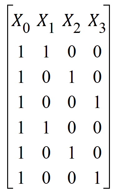
As an example, consider a simple one-way ANOVA model, with three levels. The design matrix is:

X0 is the intercept column. X1, X2, and X3 correspond to the three levels of the treatment effect. X0 and X1 are clearly linearly independent, as is X2 linearly independent of X0 and X1. But X3 is not linearly independent of X0, X1, and X2, since X3=X0 – X1 – X2. Hence b3 would be set to zero. The degrees of freedom for an effect is the number of columns remaining after this process. In this example, treatment effect has two degrees of freedom, the number typically assigned in ANOVA.
See the “Residuals worksheet and predicted values” section for computation details.
If intercept is in the model, then center the data. Perform a Gram-Schmidt orthogonalization process. If the norm of the vector after GS divided by the norm of the original vector is less than d, then the vector is called singular.
Transformation of the response
The Dependent Variables Transformation menu provides three options: No transformation, ln transformation (loge), or log transformation (log10). Transformations are applied to the response before model fitting. Note that all estimates using log will be the same estimates found using ln, only scaled by ln 10, since log(x)=ln(x)/ln(10).
If the standard deviation is proportional to the mean, taking the logarithm often stabilizes the variance, resulting in better fit. This implicitly assumes that the error structure is multiplicative with lognormal distribution.
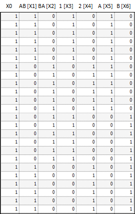
The fixed effects are given in the linear combination expression. Using that model, the design matrix X would be expanded into that presented in the following table. The vector of fixed effects corresponding to that design matrix would be: b = (b0,b1,b2,b3,b4,b5,b6).
Notice that X2=X0 – X1. Hence set b2=0. Similarly, X4=X0 – X3 and X6=X0 – X5, and hence set b4=0 and b6=0.
The table below shows the design matrix expanded for a the fixed effects model Sequence + Period +Treatment.
