WagnerNelson Object

 

The WagnerNelson model is a one-compartment IV-bolus model that uses deconvolution to estimate the fraction of drug absorption. The model also generates AUCs (Areas Under the Curve) and rate of absorption values. This deconvolution model is best used to calculate the absorption kinetics of intra­venously administered drugs.

For drugs that are administered through methods other than IV-bolus, such as oral or transdermal methods, it is preferable to use the Deconvolution object to evaluate drug release and absorption. For more information on the Deconvolution object, see “Deconvolution”.

Use one of the following to add a WagnerNelson object to a Workflow:

Right-click menu for a Workflow object: New > IVIVC > WagnerNelson 
Main menu: Insert > IVIVC > WagnerNelson.
Right-click menu for a worksheet: Send To > IVIVC > WagnerNelson.

Note:To view the object in its own window, select it in the Object Browser and double-click it or press ENTER. All instructions for setting up and execution are the same whether the object is viewed in its own window or in Phoenix view.

This section contains the following topics:

• WagnerNelson inputs and calculations

• Main panel

• Dosing panel

• Slopes Selector panel

• Slopes panel

• Options tab

• Plots tab

• Results

WagnerNelson inputs and calculations

The Wagner-Nelson method estimates the fraction of drug absorbed over time, relative to the total amount to be absorbed, following the method described in Gibaldi and Perrier (1975) pages 130 to 133. It uses as a basis AUC values computed for each time point in the time-concentration data.

Note:Wagner-Nelson computations assume single-dose PK data with a concentration value of zero at dose time. If no concentration value exists at dose time, WinNonlin will insert a concentration value of zero.

The value of AUCINF (AUC_¥) may be user-specified or WinNonlin can compute it as for non-compart­mental analysis:

Either the observed or predicted value for C_last, where C_{last_pred}=exp(intercept – Lambda_z*t_last) can be used. As in the Wagner-Nelson method, the method for computing Lambda Z is specified by the user: best fit, user-specified range, or user-specified value. An intercept for the last case can be entered by the user. If the intercept is not specified, WinNonlin will compute it using the last positive concentration and associated time value:

The cumulative amount absorbed at time t, normalized by the central compartment volume V1, is computed as:

Therefore, Cumul_Amt_Abs_V at t=infinity is:

The relative fraction absorbed at time t is then:

Data points with a missing value for either time or the concentration will be excluded from the analysis and will not appear in the output.

Main panel

Use the Main Mappings panel to identify how input variables are used in a WagnerNelson object. Required input is highlighted orange in the interface.

•None: Data types mapped to this context are not included in any analysis or output.

•Sort: Categorical variable(s) identifying individual data profiles, such as subject ID.

•Carry: Data variable(s) to include in the output worksheets.

•X: Nominal or actual time collection points in a study.

•Y: Drug concentration values from blood plasma.

Dosing panel

Note:If no concentration value exists at dose time for a given profile, Phoenix inserts a concentration value of zero at the specified dose time.

The time units for the dosing data must be the same as the time units for the time/concentration data.

•None: Data types mapped to this context are not included in any analysis or output.

•Sort: Categorical variable(s) identifying individual data profiles, such as subject ID.

•Time of Last Dose: Time of the last dose administration.

Dosing sorts dialog

The first time a user selects the Dosing panel Phoenix displays a dialog that prompts the user to select the sort variables to use to create the internal dosing worksheet. This dialog is only displayed if sort keys are selected.

 

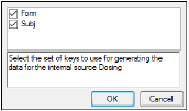
The Dosing sorts dialog uses the sort variables specified in the Main Mappings panel. By default all sort variables are selected.

• Click OK to accept the default sort variables.

• To select a subset of the sort variables, clear the checkbox beside the unwanted sort variable and click OK.

• To choose new sort variables, click Rebuild in the Dosing panel. The Dosing panel is cleared and the Dosing sorts dialog is displayed again.

Slopes Selector panel

Phoenix estimates the rate constant Lambda Z, which is associated with the terminal elimination phase for concentration data. These measurements are estimated using the linear or the linear-log trapezoidal rules, which are selected in the Calculation Method menu in the Options tab. If Lambda Z is estimable, parameters for concentration data are extrapolated to infinity.

The following section contains usage instructions. For descriptions of how the WagnerNelson model determines Lambda Z or slope estimation settings, see “Lambda Z or Slope Estimation settings”.

If the observation data does not extend significantly into the terminal phase, then selecting Observed in the Area Under the Curve menu can cause the model to significantly underestimate the actual AUCINF. For example, if the absorption phase was not completed, then scaling errors can occur when Phoenix computes the fraction absorbed.

To define the Lambda Z or slope estimation settings

• Select Slopes Selector in the Setup tab.
  
  The observed times for each profile are displayed on a graph. A graph for each profile is listed on separate tabs in the Slopes Selector panel.

• Use the View menu to select a linear (Lin) or logarithmic (Log) axis scale.

• Use the Lambda Z Calculation Method menu to select Best Fit, Time Range, or Parameters as the calculation method.

•If Best Fit is selected, Phoenix calculates the points for Lambda Z estimation for each profile.

•If Time Range is selected users must type the start and end times for Lambda Z estimation in the Start and End fields.

•If Parameters is selected users can type their own values in the Lambda Z and Intercept fields. Intercept values are optional, so if no intercept value is entered, Phoenix computes it as: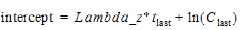

Since no specific points are used in the Lambda Z computation, the Lambda Z output in the Results tab will contain predicted and residual values for all time and concentration values. Any start times, end times, Lambda Z values, and intercept values must be greater than zero.

• In the Area Under the Curve menu, select a method to use to calculate the AUC to time=infinity.

•If Predicted is selected, then Phoenix calculates the area under the curve (AUC) as AUC_¥=AUC_last+C_last/Lambda_z, where C_last is the last predicted concentration.

•If Observed is selected, then Phoenix calculates the AUC as AUC_¥=AUC_last+C_last/Lamb­da_z, where C_last is the last observed concentration.

•If Specified is selected, then users can type a value for the AUC in the specified values field. The AUC value must be greater than zero.

Caution:If Specified is selected in the Area Under the Curve menu, then any user-specified Lambda Z Calculation Method settings are not applied to the Loo-Riegelman model results.

To set start times, end times, and exclusions

Users can manually select start times, end times, and excluded time points by selecting them on each profile graph.

Note:Manually selecting times and exclusions automatically sets the Lambda Z Calculation Method to Time Range.

• Left-click a data point on a graph to select the start time.

• Press SHIFT and left-click a data point on a graph to select the end time.

• Press CTRL and left-click a data point on a graph to exclude the time point.

• Remove or change the start time, end time, and exclusions by selecting new points on the graph using the same mouse and keyboard commands listed in steps 1 through 3.

When the start time, end time, and exclusions are manually selected, the graph title is updated to show the new R² calculation, the graph is updated to show the new slope, and the legend is updated to show the new slope and exclusions, as shown below.

 

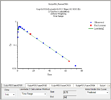
Manually selected start, end, and excluded time points for the first profile

Note:Excluded data points apply only to Lambda Z or slope calculations. The excluded data points are still included in the computation of AUCs, moments, etc.

Slopes panel

In the Slopes panel, users can enter the start times, end times, and exclusions used to calculate the Lambda Z for each profile defined in the Slopes panel. Users can also enter AUC_¥ values, select the AUC computation method, enter Lambda Z and intercept values, and select the Lambda Z calculation method.

Users can type their own values and select calculation methods in the Slopes panel. The following section contains usage instructions. For descriptions of how the WagnerNelson model determines Lambda Z or slope estimation settings, see “Lambda Z or Slope Estimation settings”.

To define slopes and select calculation methods

• Select Slopes in the Setup tab.

• Type the start and end time values in the Start Time and End Time columns for each profile.

• Type excluded time points in the Exclusions column for each profile.
  Exclude multiple time points for a profile by typing the time points in the same cell and separating the time points with a semicolon.

• Type user-specified AUC_¥ values in the AUCINF column. The value must be greater than zero.

• Select an AUC calculation method in the AUC Method column.

• Type Lambda Z values in the LambdaZ column.

• Type slope intercept values in the *Intercept column.
  
  Slope intercept values are optional. If no intercept value is entered, Phoenix computes it as: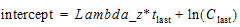

• Select a Lambda Z calculation method in the Fit Method column.

To apply slope and calculation settings to multiple profiles

• Type the desired start and end times, exclusions, and other values and select the calculation methods for the first profile or profile group.

• When all changes are made, use the pointer to highlight all the rows for every column between Start Time and Fit Method columns for the first profile or profile group.

• Place the pointer over the black square on the lower right side of the selection. The pointer changes to the following shape. This signifies that the drag and fill feature can be used.

 

• Press the left mouse button and drag the selection down to fill the InVitro Estimates cells beside each formulation.

To copy the same settings from one profile to another

• Enter all necessary values and select the calculation methods for a profile.

• Use the pointer to highlight the entire row.

• The pointer changes to the following shape. This signifies that the drag feature can be used.

 

• Press the left mouse button to drag the target row of slope settings to the destination row.

Example column headings for Slopes table:

•Sort variable(s): Categorical variable(s) identifying individual data profiles, such as subject ID. The sort variables selected in the Main Mappings panel are used as default column head­ings. In the previous image, Subj is the sort variable.

•Start Time: Users must type the start and end times for Lambda Z estimation in the Start and End fields.

•End Time: Users must type the start and end times for Lambda Z estimation in the Start and End fields.

•Exclusions: Excluded data points in the plots.

•AUCINF: User-specified AUCINF values. The values must be greater than zero.

•AUC Method: Select a method to use to calculate the AUC to time=infinity.

•LambdaZ: Users can type their own values in the LambdaZ and Intercept fields. Intercept values are optional, so if no intercept value is entered, Phoenix computes it as: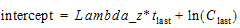

•Intercept: Y-intercept value. Entering this value is optional.

•Fit Method: Select Best Fit, Time Range, or Parameters as the Lambda Z calculation method.

Options tab

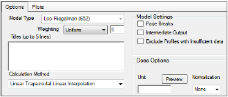
The Options tab allows users to select the WagnerNelson model and set options for the selected model.

 

• Use the Weighting menu to select the regression that estimates Lambda Z or slopes. Available options include:

•User Defined

•Uniform

•1/Y

•1/(Y*Y)

Note:The relative proportions of the weights are important, not the weights themselves. See “Weighting” in the WinNonlin NCA section for more on weighting schemes.

When selecting a weighting model, there are a couple of rules to consider:

If User Defined is selected then users can enter their own Observed to Power N value. The value of N must be typed in the Weighting text field.

When a log-linear fit is done (Uniform weighting for Lambda Z), then the fit is implicitly using a weighting approximately equal to 1/Yhat².

Note:If 1/Y and the Linear Log Trapezoidal calculation method are selected, a user could assume that the weighting scheme is 1/LogY, rather than 1/Y. However, this is not the case because concentra­tions between zero and one would have negative weights, and could not be included in the analy­sis.

• Use the Titles text box to type a title for the analysis.
  
  The title is displayed at the top of each page in the Core output. The title can include up to five lines of text.

• Use the Calculation Method menu to select a calculation method.
  
  Four methods are available for the calculation of area under the curve. The chosen method applies to all AUC and AUMC computations. All methods reduce to the log trapezoidal rule, the linear trapezoidal rule, or both. The methods differ based on when the rules are applied. See “Partial area calculation” for descriptive equations of the calculation methods.

•Linear_Log_Trapezoidal: uses the log trapezoidal rule after Cmax, or after C0 if C0 > Cmax. Otherwise the linear trapezoidal rule is used. If Cmax is not unique, then the first maximum is used. This method uses linear trapezoids before Tmax and log trapezoids after Tmax.

•Linear_Trapezoidal_Linear_Interpolation: This is the default method. It applies the linear trapezoidal rule to each pair of consecutive points in the dataset that have non-missing val­ues, and sums up these areas. This method uses linear trapezoids before and after Tmax.

•Linear_Up_Log_Down: uses the linear trapezoidal rule any time that the concentration data is increasing, and the logarithmic trapezoidal rule is used any time that the concentration data is decreasing. This method uses linear trapezoids up and logarithmic trapezoids down before Tmax and linear trapezoids up and logarithmic trapezoids down after Tmax.

•Linear_Trapezoidal_LinearLog_Interpolation: this method is the same as Linear_Trape­zoidal_Linear_Interpolation. It is used when a final time point, that is not in the dataset, is used for predictions. In that case, Phoenix inserts a final concentration value using the Lin­ear_Trapezoidal_Linear_Interpolation rule. If the final time point is after Cmax, or after C0 if C0 > Cmax, the Linear_Trapezoidal_LinearLog_Interpolation rule is used. If Cmax is not unique, then the first maximum is used. This method uses linear trapezoids before and after Tmax.

Note:The Linear Log Trapezoidal, the Linear Up Log Down, and the Linear Trapezoidal Linear/Log Interpolation methods all apply the same exceptions in area calculation and interpolation. If a Y value (concentration, rate, or effect) is less than or equal to zero, Phoenix defaults to the linear trapezoidal or linear interpolation rule for that point. If adjacent Y values are equal to each other, Phoenix defaults to the linear trapezoidal or linear interpolation rule.

No interpolation is performed in the Loo-Riegelman model.

• Select the Page Breaks checkbox to include page breaks in the text output.

• Select the Intermediate Output checkbox to set text output to only include values for iterations during estimation of Lambda Z or slopes, and for each of the sub-areas in partial area computa­tions.

• Select the Exclude Profiles with Insufficient data checkbox to exclude profiles with all or many missing parameter estimates from the results.
  
  If this option is not selected, profiles with insufficient data will have missing output parameter val­ues. See “Data deficiencies resulting in missing values for PK parameters” for a list of cases that produce missing estimates and are excluded by selecting this option.

To set the dosing unit

• Type the dosing unit into the Unit field.

• Click Preview to see a preview of dose option selections.
  The preview is opened in its own window. Click OK to close the preview window.

• Use the Normalization menu to select the appropriate factor if the dose amount is normalized by subject body weight or body mass index. Normalization menu options include:

•None 

•kg 

•g 

•mg 

•m**2 

•1.73 m**2 

If doses are in milligrams per kilogram of body weight, select mg as the dosing unit and kg as the dose normalization. The Normalization menu affects the output parameter units. For example, if dose volume is in liters, selecting kg as the dose normalization changes the units to L/kg. Dose normalization affects units for all volume and clearance parameters, as well as AUCinf/D values.

Plots tab

In the Plots tab, users can select whether or not to produce plot output.

 

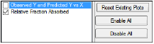
• Use the checkboxes to toggle the creation of graphs.

• Click Reset Existing Plots to clear all existing plot output.
  
  Each plot in the Results tab is a single plot object. Every time a model is executed, each object remains the same, but the values used to create the plot are updated. This way, any styles that are applied to the plots are retained no matter how many time the model is executed.
  
  Clicking Reset Existing Plots removes the plot objects from the Results tab, which clears any custom changes made to the plot display.

• Use the Enable All and Disable All buttons to check or clear all checkboxes for all plots in the list. These buttons are most useful when there are many plots listed.

Results

 

Users can double-click a plot in the Results tab to edit it. (See the menu options descriptions in the Plots chapter of the Data Tools and Plots Guide for plot editing options.)

 

---

Last modified date:6/26/19

Legal Notice | Contact Certara
© 2019 Certara USA, Inc. All rights reserved.