Deconvolution is used to evaluate in vivo drug release and delivery when data from a known drug input are available. Phoenix’s Deconvolution object can estimate the cumulative amount and fraction absorbed over time for individual subjects, using PK profile data and dosing data per profile.
Use one of the following to add the Deconvolution object to a Workflow:
Right-click menu for a Workflow object: New > NCA and Toolbox > Deconvolution.
Main menu: Insert > NCA and Toolbox > Deconvolution.
Right-click menu for a worksheet: Send To > NCA and Toolbox > Deconvolution.
Note:To view the object in its own window, select it in the Object Browser and double-click it or press ENTER. All instructions for setting up and execution are the same whether the object is viewed in its own window or in Phoenix view.
Use the Main Mappings panel to identify how input variables are used in the Deconvolution object. Deconvolution requires a dataset containing time and concentration data, and sort variables to identify individual profiles. Required input is highlighted orange in the interface.
•None: Data types mapped to this context are not included in any analysis or output.
•Sort: Categorical variable(s) identifying individual data profiles, such as subject ID in a deconvolution analysis. A separate analysis is performed for each unique combination of sort variables.
•Time: The relative or nominal dosing times used in a study.
•Concentration: The measured amount of a drug in blood plasma.
The Deconvolution object assumes a unit impulse response function (UIR) of the form:
|
|
(1) |
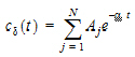
where N is the number of exponential terms.
Use the Exponential Terms panel to enter values for the A and alpha parameters. For oral administration, the user should enter values such that:
|
|
(2) |

Required input is highlighted orange in the interface.
•None: Data types mapped to this context are not included in any analysis or output.
•Sort: Categorical variable(s) identifying individual data profiles, such as subject ID.
•Parameter: Data variable(s) to include in the output worksheets.
•Value: A (coefficients) and Alpha (exponential) parameter values.
A and alpha parameters are listed sequentially based on the number of exponential terms selected. If only one exponential term is selected, each profile has an A1 and an Alpha1 parameter. If two exponential terms are selected, each profile has an A1 and an A2 parameter, and an Alpha1 and an Alpha2 parameter.
Rules for using an external exponential terms worksheet:
-
The sort variables must match the sort variables used in the main input dataset.
-
The worksheet’s parameter column must match the number of exponential terms selected in the Exponential Terms menu. For example, if three exponential terms are selected, then each profile in the exponential terms worksheet must have three A parameters and three alpha parameters.
-
The units used for the A and alpha parameters must match the units used for the concentration and dosing data. For example, If the concentration data has units ng/mL and the dosing data has units mg, then the A units must be ng/mL/mg, or the input data or dosing data should be converted (using Data Wizard Properties) to have consistent units. If the time units are hr, then the alpha units are 1/hr.
-
If the UIR parameters are unknown, but a dataset is available that represents the impulse response, the parameters can be estimated by fitting the data in Phoenix with PK model 1, 8, or 18 (for N=1, 2, or 3, respectively). Since the UIR is the response to one dose unit, for model 1 (one-compartment), the inverse of the model parameter V is used for the UIR parameter, i.e., A1=1/V. For model 8 (two-compartment), the model parameters A and B should be divided by the stripping dose to obtain A1 and A2 for the UIR, and similarly for model 18 (three-compartment). However, if the dose units are different than the concentration mass units, the ‘A’ parameters must be adjusted so that the units are in concentration units divided by dose units. For the example in the prior bullet, if A=1/V from model 1 has units 1/mL, then ‘A’ must be converted to ng/mL/mg before it is used for the UIR in the Deconvolution object, A=10^6/V.
Supplying dosing information using the Dose panel is optional. Without it, the Deconvolution object runs correctly by assuming a dose at time zero time-concentration data with the fraction absorbed approaching a final value of one. The dose time is assumed to be zero for all profiles.
Note:The sort variables in the dosing data worksheet must match the sort variables used in the main input dataset.
Required input is highlighted orange in the interface.
•None: Data types mapped to this context are not included in any analysis or output.
•Sort: Categorical variable(s) identifying individual data profiles, such as subject ID.
•Dose: The amount of drug administered.
If the Use times from a worksheet column option button is selected in the Options tab, then the Observed Times panel is displayed in the Setup list. Required input is highlighted orange in the interface.
•None: Data types mapped to this context are not included in any analysis or output.
•Time: Time values.
•Sort: Sort variables.
Note:The observed times worksheet cannot contain more than 1001 time points.
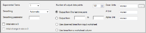
The Options tab allows users to specify settings for exponential terms, parameters, and output time points.
-
In the Exponential Terms menu, select the number of exponential terms in the unit impulse response to use per profile (up to nine exponential terms can be added).
-
In the Smoothing menu, select the method Phoenix uses to determine the dispersion parameter.
•Automatic tells Phoenix to find the optimal value for the dispersion parameter delta.
•None disables smoothing that comes from the dispersion function. If selected, the input function is the piecewise linear precursor function.
•User allows users to type the value of the dispersion parameter delta as the smoothing parameter. The delta value must be greater than zero. Increasing the delta value increases the amount of smoothing.
-
In the Smoothing parameter field, enter the value for the smoothing parameter.
This option is only available if User is selected in the Smoothing menu. -
Select the Initial rate is 0 checkbox to set the estimated input rate to zero at the initial time or lag time.
-
Select the Initial Change in Rate is 0 checkbox to set the derivative of the estimated input rate to zero at the initial time or lag time.
This option is only available if the Initial rate is 0 checkbox is selected. -
In the Dose Units field, type the dosing units to use with the dataset.
•Click the Units Builder  button to use the Units Builder dialog to add dosing units.
•See “Using the Units Builder” for more details on this tool.
-
In the Number of output data points box, type or select the number of output data points to use per profile.
The maximum number of time points allowed is 1001. -
Select the Output from 0 to last time point option button to have Phoenix generate output at even intervals from time zero to the final input time point for each profile.
-
Select the Output from _ to _ option button to have Phoenix generate output at even intervals between user-specified time points for each profile.
•Type the start time point in the first field and type the end time point in the last field.
-
Select the Use observed times from input worksheet option button to have Phoenix generate output at each time point in the input dataset for each profile.
-
Select the Use times from a worksheet column option button to use a separate worksheet to provide in vivo time values.
•Selecting this option creates an extra panel called Observed Times in the Setup tab list.
•Users must map a worksheet containing time values used to generate output data points to the Observed Times panel.
•The observed times worksheet cannot contain more than 1001 time points.
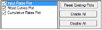
The Plots tab allows users to select whether or not plots are included in the output.
-
Use the checkboxes to toggle the creation of graphs.
-
Click Reset Existing Plots to clear all existing plot output.
Each plot in the Results tab is a single plot object. Every time a model is executed, each object remains the same, but the values used to create the plot are updated. This way, any styles that are applied to the plots are retained no matter how many time the model is executed.
Clicking Reset Existing Plots removes the plot objects from the Results tab, which clears any custom changes made to the plot display. -
Use the Enable All and Disable All buttons to check or clear all checkboxes for all plots in the list. These buttons are most useful when there are many plots listed.
The Deconvolution object generates worksheets, plots, and a text file.
|
Worksheet |
Content |
|
Fitted Values |
Predicted data for each profile. |
|
Parameters |
The smoothing parameter delta and absorption lag time for each profile. |
|
Values |
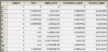
Time, input rate, cumulative amount (Cumul_Amt, using the dose units) and fraction input (Cumul_Amt/test dose or, if no test doses are given, then fraction input approaches one) for each profile. |
The Deconvolution object creates three plots for each profile. Each plot is displayed on its own page in the Results tab.
Select each plot in the Results tab. Click the page tabs at the bottom of each plot panel to view the plots for individual profiles.
|
Plot |
Content |
|
Cumulative Rates |
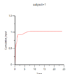
Cumulative drug input vs. time. |
|
Fitted Curves |
Observed time-concentration data vs. the predicted curve. |
|
Input Rates |
Rate of drug input vs. time. |
Users can double-click any plot in the Results tab to edit it. (See the menu options discussion in the Plots chapter of the Data Tools and Plots Guide for plot editing options.)
The Deconvolution object also creates a text file called Settings.
|
Text file |
Content |
|
Settings |
Input settings for smoothing, number of output points and start and end times for output. |
Deconvolution is used to evaluate in vivo drug release and delivery when data from a known drug input are available. Depending upon the type of reference input information available, the drug transport evaluated will be either a simple in vivo drug release such as gastro-intestinal release, or a composite form, typically consisting of an in vivo release followed by a drug delivery to the general systemic circulation.
One common deconvolution application is the evaluation of drug release and drug absorption from orally administered drug formulations. In this case, the bioavailability of the drug is evaluated if the reference formulation uses vascular drug input. Similarly, gastro-intestinal release is evaluated if the reference formulation is delivered orally. However, the Deconvolution object can also be used for other types of delivery, including transdermal or implant drug release and delivery.
Deconvolution provides automatic calculation of the drug input. It also allows the user to direct the analysis to investigate issues of special interest through different parameter settings and program input.
The methodology is based on linear system analysis with linearity defined in the general sense of the linear superposition principle. It is well recognized that classical linear compartmental kinetic models exhibit superposition linearity due to their origin in linear differential equations. However, all kinetic models defined in terms of linear combinations of linear mathematical operators, such as differentiation, integration, convolution, and deconvolution, constitute linear systems adhering to the superposition principle. The scope and generality of the linear system approach ranges far beyond linear compartmental models.
To fully appreciate the power and generality of the linear system approach, it is best to depart from the typical, physically structured modeling view of pharmacokinetics. To cut through all the complexity and objectively deal with the present problems, it is best to consider the kinetics of drug transport in a non-parametric manner and simply use stochastic transport principles in the analysis.
Convolution/deconvolution — stochastic background
The convolution/deconvolution principles applied to evaluate drug release and drug input (absorption) can be explained in terms of point A to point B stochastic transport principles. For example, consider the entry of a single drug molecule at point A at time zero. Let B be a sampling point (a given sampling space or volume) anywhere in the body (e.g. a blood sampling) that can be reached by the drug molecule entering at A. The possible presence of the molecule at B at time t is a random variable due to the stochastic transport principles involved. Imagine repeating this one molecule experiment an infinite number of times and observing the fraction of times that the molecule is at B at time t. That fraction represents the probability that a molecule is at point B given that it entered point A at time zero. Denote this probability by the function g(t).
Next, consider a simultaneous entry of a very large number (N) of drug molecules at time zero, like in a bolus injection. Let it be assumed that there is no significant interaction between the drug molecules, such that the probability of a drug molecule's possible arrival at sampling site B is not significantly affected by any other drug molecule. Then the transport to sampling site B is both random and independent. In addition the probability of being at B at time t is the same and equals g(t) for all of the molecules. It is this combination of independence and equal probability that leads to the superposition property that in its most simple form reveals itself in terms of dose-proportionality. For example, in the present case the expected number of drug molecules to be found at sampling site B at time t (NB(t)) is equal to Ng(t). It can be seen from this that the concentration of drug at the sampling site B at the arbitrary time t is proportional to the dose. N is proportional to the dose and g(t) does not depend on the dose due to the independence in the transport.
Now further assume that the processes influencing transport from A to B are constant over time. The result is that the probability of being at point B at time t depends on the elapsed time since entry at A, but is otherwise independent of the entry time. Thus the probability of being at B for a molecule that enters A at time tA is g(t – tA). This assumed property is called time-invariance. Consider again the simultaneous entry of N molecules, but now at time tA instead of zero. Combining this property with those of independent and equal probabilities, i.e., superposition, results in an expected number of molecules at B at time t given by NB(t)=Ng(t – tA).
Suppose that the actual time at which the molecule enters point A is unknown. It is instead a random quantity tA distributed according to some probability density function h(t), that is,
|
|
(3) |
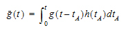
The probability that such a molecule is at point B at time t is the average or expected value of g(t – tA) where the average is taken over the possible values of tA according to:
|
|
(4) |

Causality dictates that g(t) must be zero for any negative times, that is, a molecule cannot get to B before it enters A. For typical applications drug input is restricted to non-negative times so that h(t)=0 for t < 0. As a result the quantity g(t –tA)h(tA) is nonzero only over the range from zero to t and the equation becomes:
|
|
(5) |
Suppose again that N molecules enter at point A but this time they enter at random times distributed according to h(t). This is equivalent to saying that the expected rate of entry at A is given by N’A (t)=Nh(t). As argued before, the expected number of molecules at B at time t is the product of N and the probability of being at B at time t, that is,
|
|
(6) |

Converting from number of molecules to mass units:
|
|
(7) |
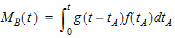
where MB(t) is the mass of drug at point B at time t and f(t) is the rate of entry in mass per unit time into point A at time t.
Let Vs denote the volume of the sampling space (point B). Then the concentration, c(t), of drug at B is:
|
|
(8) |
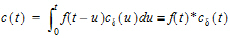
where “*” is used to denote the convolution operation and
|
|
(9) |
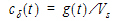
The above equation is the key convolution equation that forms the basis for the evaluation of the drug input rate, f(t). The function cd(t) is denoted as the unit impulse response, also known as the characteristic response or the disposition function. The process of determining the input function f(t) is called deconvolution because it is required to deconvolve the convolution integral in order to extract the input function that is embedded in the convolution integral.
The unit impulse response function (cd) provides the exact linkage between drug level response c(t) and the input rate function f(t). cd is simply equal to the probability that a molecule entering point A at t=0 is present in the sampling space at time t divided by the volume of that sample space.
Phoenix models the input function as a piecewise linear “precursor” function fp(t) convolved with an exponential “dispersion” function fd(t). The former provides substantial flexibility whereas the latter provides smoothness. The piecewise linear component is parameterized in terms of a sum of hat-type wavelet basis functions, hj(t):
|
|
(10) |
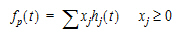
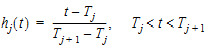
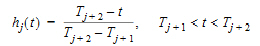
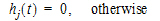
where xj is the dose scaling factor within a particular observation interval and Tj are the wavelet support points. The hat-type wavelet representation enables discontinuous, finite duration drug releases to be considered together with other factors that result in discontinuous delivery, such as stomach emptying, absorption window, pH changes, etc. The dispersion function provides the smoothing of the input function that is expected from the stochastic transport principles governing the transport of the drug molecules from the site of release to subsequent entry to and mixing in the general systemic circulation.
The wavelet support points (Tj) are constrained to coincide with the observation times, with the exception of the very first support point that is used to define the lag-time, if any, for the input function. Furthermore, one support point is injected halfway between the lag-time and the first observation. This point is simply included to create enough capacity for drug input prior to the first sampling. Having just one support point prior to the first observation would limit this capacity. The extra support point is well suited to accommodate an initial “burst” release commonly encountered for many formulations.
The dispersion function fd(t) is defined as an exponential function:
|
|
(11) |
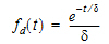
where d is denoted the dispersion or smoothing parameter. The dispersion function is normalized to have a total integral (t=0 to ¥) equal one, which explains the scaling with the d parameter. The input function, f(t), is the convolution of the precursor function and the dispersion function:
|
|
(12) |
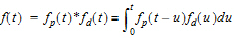
The general convolution form of the input function above is consistent with stochastic as well as deterministic transport principles. The drug level profile, c(t), resulting from the above input function is, according to the linear disposition assumption, given by:
|
|
(13) |
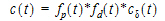
where “*” is used to denote the convolution operation.
Deconvolution through convolution methodology
Phoenix deconvolution uses the basic principle of deconvolution through convolution (DTC) to determine the input function. The DTC method is an iterative procedure consisting of three steps. First, the input function is adjusted by changing its parameter values. Second, the new input function is convolved with cd(t) to produce a calculated drug level response. Third, the agreement between the observed data and the calculated drug level data is quantitatively evaluated according to some objective function. The three steps are repeated until the objective function is optimized. DTC methods differ basically in the way the input function is specified and the way the objective function is defined. The objective function may be based solely on weighted or unweighted residual values, or observed–calculated drug levels. The purely residual-based DTC methods ignore any behavior of the calculated drug level response between the observations.
The more modern DTC methods, including Phoenix’s approach, consider both the residuals and other properties such as smoothness of the total fitted curve in the definition of the objective function. The deconvolution method implemented in Phoenix is novel in the way the regularization (smoothing) is implemented. Regularization methods in some other deconvolution methods are done through a penalty function approach that involves a measurement of the smoothness of the predicted drug level curve, such as the integral of squared second derivative.
The Phoenix deconvolution method instead introduces the regularization directly into the input function through a convolution operation with the dispersion function, fd(t). In essence, a convolution operation acts like a “washout of details”, that is a smoothing due to the mixing operation inherent in the convolution operation. Consider, for example, the convolution operation that leads to the drug level response c(t). Due to the stochastic transport principles involved, the drug level at time t is made up of a mixture of drug molecules that started their journey to the sampling site at different times and took different lengths of time to arrive there. Thus, the drug level response at time t depends on a mixture of prior input. It is exactly this mixing in the convolution operation that provides the smoothing. The convolution operation acts essentially as a low pass filter with respect to the filtering of the input information. The finer details, or higher frequencies, are attenuated relative to the more slowly varying components, or low frequency components.
Thus, the convolution of the precursor function with the dispersion function results in an input function, f(t), that is smoother than the precursor function. Phoenix allows the user to control the smoothing through the use of the smoothing parameter d. Decreasing the value of the dispersion function parameter d results in a decreasing degree of smoothing of the input function. Similarly, larger values of d provide more smoothing. As d approaches zero, the dispersion function becomes equal to the so-called Dirac delta “function”, resulting in no change in the precursor function.
The smoothing of the input function, f(t), provided by the dispersion function, fd(t), is carried forward to the drug level response in the subsequent convolution operation with the unit impulse response function (cd). Smoothing and fitting flexibility are inversely related. Too little smoothing (too small a d value) will result in too much fitting flexibility that results in a “fitting to the error in the data.” In the most extreme case, the result is an exact fitting to the data. Conversely, too much smoothing (too large a d value) results in too little flexibility so that the calculated response curve becomes too “stiff” or “stretched out” to follow the underlying true drug level response.
Phoenix's deconvolution function determines the optimal smoothing without actually measuring the degree of smoothing. The degree of smoothing is not quantified but is controlled through the dispersion function to optimize the “consistency” between the data and the estimated drug level curve. Consistency is defined here according to the cross validation principles. Let rj denote the differences between the predicted and observed concentration at the j-th observation time when that observation is excluded from the dataset. The optimal cross validation principle applied is defined as the condition that leads to the minimal predicted residual sum of squares (PRESS) value, where PRESS is defined as:
|
|
(14) |
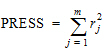
For a given value of the smoothing parameter d, PRESS is a quadratic function of the wavelet scaling parameters x. Thus, with the non-negativity constraint, the minimization of PRESS for a given d value is a quadratic programming problem. Let PRESS (d) denote such a solution. The optimal smoothing is then determined by finding the value of the smoothing parameter d that minimizes PRESS (d). This is a one variable optimization problem with an embedded quadratic-programming problem.
Phoenix's deconvolution function permits the user to override the automatic smoothing by manual setting of the smoothing parameter. The user may also specify that no smoothing should be performed. In this case the input rate function consists of the precursor function alone.
Besides controlling the degree of smoothing, the user may also influence the initial behavior of the estimated input time course. In particular the user may choose to constrain the initial input rate to zero (f(0)=0) and/or constrain the initial change in the input rate to zero (f'(0)=0). By default Phoenix does not constrain either initial condition. Leaving f(0) unconstrained permits better characterization of formulations with rapid initial “burst release,” that is, extended release dosage forms with an immediate release shell. This is done by optionally introducing a bolus component or “integral boundary condition” for the precursor function so the input function becomes:
|
f(t)=fp(t)*fd(t)+xd fd(t) |
(15) |
where the fp(t)*fd(t) is defined as before.
The difference here is the superposition of the extra term xd fd(t) that represents a particularly smooth component of the input. The magnitude of this component is determined by the scaling parameter xd, which is determined in the same way as the other wavelet scaling parameters previously described.
The estimation procedure is not constrained with respect to the relative magnitude of the two terms of the composite input function given above. Accordingly, the input can “collapse” to the “bolus component” xd fd(t) and thus accommodate the simple first-order input commonly experienced when dealing with drug solutions or rapid release dosage forms. A drug suspension in which a significant fraction of the drug may exist in solution should be well described by the composite input function option given above. The same may be the case for dual release formulations designed to rapidly release a portion of the drug initially and then release the remaining drug in a prolonged fashion. The prolonged release component will probably be more erratic and would be described better by the more flexible wavelet-based component fp(t)*fd(t) of the above dual input function.
Constraining the initial rate of change to zero (f'(0)=0) introduces an initial lag in the increase of the input rate that is more continuous in behavior than the usual abrupt lag time. This constraint is obtained by constraining the initial value of the precursor function to zero (fp(0)=0). When such a constrained precursor is convolved with the dispersion function, the resulting input function has the desired constraint.
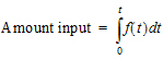
The extent of drug input in the Deconvolution object is presented in two ways. First, the amount of drug input is calculated as:
|
|
(16) |
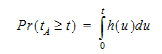
Second, the extent of drug input is given in terms of fraction input. If test doses are not supplied, the fraction is defined in a non-extrapolated way as the fraction of drug input at time t relative to the amount input at the last sample time, tend:
|
|
(17) |
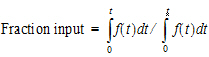
The above fraction input will by definition have a value of one at the last observation time, tend. This value should not be confused with the fraction input relative to either the dose or the total amount absorbed from a reference dosage form. If dosing data is entered by the user, the fraction input is relative to the dose amount (i.e., dose input on the dosing sheet).
Charter and Gull (1987). J Pharmacokinet Biopharm 15, 645–55.
Cutler (1978). Numerical deconvolution by least squares: use of prescribed input functions. J Pharmacokinet Biopharm 6(3):227–41.
Cutler (1978). Numerical deconvolution by least squares: use of polynomials to represent the input function. J Pharmacokinet Biopharm 6(3):243–63.
Daubechies (1988). Orthonormal bases of compactly supported wavelets. Communications on Pure and Applied Mathematics 41(XLI):909–96.
Gabrielsson and Weiner (2001). Pharmacokinetic and Pharmacodynamic Data Analysis: Concepts and Applications, 3rd ed. Swedish Pharmaceutical Press, Stockholm.
Gibaldi and Perrier (1975). Pharmacokinetics. Marcel Dekker, Inc, New York.
Gillespie (1997). Modeling Strategies for In Vivo-In Vitro Correlation. In Amidon GL, Robinson JR and Williams RL, eds., Scientific Foundation for Regulating Drug Product Quality. AAPS Press, Alexandria, VA.
Haskel and Hanson (1981). Math. Programs 21, 98–118.
Iman and Conover (1979). Technometrics, 21,499–509.
Loo and Riegelman (1968). New method for calculating the intrinsic absorption rate of drugs. J Pharmaceut Sci 57:918.
Madden, Godfrey, Chappell MJ, Hovroka R and Bates RA (1996). Comparison of six deconvolution techniques. J Pharmacokinet Biopharm 24:282.
Meyer (1997). IVIVC Examples. In Amidon GL, Robinson JR and Williams RL, eds., Scientific Foundation for Regulating Drug Product Quality. AAPS Press, Alexandria, VA.
Polli (1997). Analysis of In Vitro-In Vivo Data. In Amidon GL, Robinson JR and Williams RL, eds., Scientific Foundation for Regulating Drug Product Quality. AAPS Press, Alexandria, VA.
Treitel and Lines (1982). Linear inverse — theory and deconvolution. Geophysics 47(8):1153–9.
Verotta (1990). Comments on two recent deconvolution methods. J Pharmacokinet Biopharm 18(5):483–99.
Perhaps the most common application of deconvolution is in the evaluation of drug release and drug absorption from orally administered drug formulations. In this case, the bioavailability is evaluated if the reference input is a vascular drug input. Similarly, gastrointestinal release is evaluated if the reference is an oral solution (oral bolus input). Both are included here.
This example uses the dataset M3tablet.dat, which is located in the Phoenix examples directory. The analysis objectives are to estimate the following for a tablet formulation:
Knowledge of how to do basic tasks using the Phoenix interface, such as creating a project and importing data, is assumed.
•Absolute bioavailability and rate and cumulative extent of absorption over time (see “Evaluate absolute bioavailability”)
•In vivo dissolution and the rate and cumulative extent of release over time (see “Estimate dissolution”)
The completed project (Deconvolution.phxproj) is available for reference in …\Examples\WinNonlin.
Evaluate absolute bioavailability
To estimate the absolute bioavailability, the mean unit impulse response parameters A and alpha have already been estimated from concentration-time data following instantaneous input (IV bolus) for three subjects, using PK model 1. The data in M3tablet.dat includes those parameter estimates and plasma drug concentrations following oral administration of a tablet formulation. This example shows how to estimate the rate at which the drug reaches the systemic circulation, using deconvolution.
For this type of data, all the data for one treatment must be displayed in the first rows, followed by all the data for the other treatment.
-
From within an open project, import the file …\Examples\WinNonlin\Supporting files\M3tablet.dat.
-
Right-click Workflow in the Object Browser and select New > NCA and Toolbox > Deconvolution.
-
Drag the M3tablet worksheet from the Data folder to the Main Mappings panel.
Map subject to the Sort context.
Leave time mapped to the Time context.
Map conc to the Concentration context.
Leave all the other data types mapped to None. -
Select Exp Terms in the Setup list.
-
Select the Use Internal Worksheet checkbox.
-
In the Value column type 100 for each row with A1 in the Parameter column.
-
In the Value column type 0.98 for each row with Alpha1 in the Parameter column.
There are no dose amounts for this example. The calculated fractional input approaches a value of 1 rather than being adjusted for dose amount. -
Click
 to execute the object. The results are displayed on the Results tab.
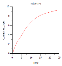
Phoenix generates worksheets and plots for the output. Partial results for subject 1 are displayed below. -
Select Cumulative Rates Plot in the Results list.
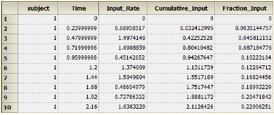
Part of the Values worksheet
To estimate the in vivo dissolution from the tablet formulation, the mean unit impulse response parameters A and alpha have already been estimated from concentration-time data following instantaneous input into the gastrointestinal tract by administration of a solution, using PK model 3. The steps below show how to use deconvolution to estimate the rate at which the drug dissolves.
For the rest of this example an oral solution (oral bolus) is used to estimate the unit impulse response. In this case, the deconvolution result should be interpreted as an in vivo dissolution profile, not as an absorption profile. The oral impulse response function should have the property of the initial value being equal to zero, which implies that the sum of the ‘A’s must be zero. The alphas should all still be positive, but at least one A will be negative.
-
Right-click Workflow in the Object Browser and select New > NCA and Toolbox > Deconvolution.
-
Drag the M3tablet worksheet from the Data folder to the Main Mappings panel.
Map subject to the Sort context.
Leave time mapped to the Time context.
Map conc to the Concentration context.
Leave all the other data types mapped to None. -
In the Options tab below the Setup panel, select 2 in the Exponential Terms menu.
-
Select Exp Terms in the Setup list.
-
Check the Use Internal Worksheet checkbox.
-
Fill in the Value column as follows:
Type -110 for each row with A1 in the Parameter column.
Type 110 for each row with A2 in the Parameter column.
Type 3.8 for each row with Alpha1 in the Parameter column.
Type 0.10 for each row with Alpha2 in the Parameter column. -
Click
 to execute the object. The results are displayed on the Results tab.
Results for subject 1 are displayed below: -
Select Cumulative Rates Plot under Plots in the Results list.
This concludes the Deconvolution example.
