Computational rules for the NCA engine are discussed in sections:
•Time deviations in steady-state data
•Data checking and pre-treatment
WinNonlin NCA computations are covered under the headings:
•Lambda Z or Slope Estimation settings
Time deviations in steady-state data
When using steady-state data, Phoenix computes AUC_TAU from dose time to dose time+tau, based on the tau value set in the Dosing panel. However, in most studies, there are sampling time deviations. For example, if dose time=0 and tau=24, the last sample might be at 23.975 or 24.083 hours. In this instance, the program will estimate the AUC_TAU based on the estimated concentration at 24 hours, and not the concentration at the actual observation time. For steady state data, Cmax, Tmax, Cmin and Tmin are found using observations taken at or after the dose time, but no later than dose time+tau.
Data checking and pre-treatment
Prior to calculation of pharmacokinetic parameters, Phoenix institutes a number of data-checking and pre-treatment procedures as follows.
-
Sorting: Prior to analysis, data within each profile is sorted in ascending time order. (A profile is identified by a unique combination of sort variable values.)
-
Inserting initial time points: If a PK profile does not contain an observation at dose time, Phoenix inserts a value using the following rules. (Note that, if there is no dosing time specified, the dosing time is assumed to be zero.)
•Extravascular and Infusion data: For single dose data, a concentration of zero is used; for steady-state, the minimum observed during the dose interval (from dose time to dose time +tau) is used.
•IV Bolus data: Phoenix performs a log-linear regression of first two data points to back-extrapolate C0. If the regression yields a slope >= 0, or at least one of the first two y-values is zero, or if one or both of the points is viewed as an outlier and excluded from the Lambda Z regression, then the first observed y-value is used as an estimate for C0. If a weighting option is selected, it is used in the regression.
•Urine data: A rate value of zero is used at dose time.
•Drug Effect data: An effect value equal to the user-supplied baseline is inserted at dose time (assumed to be zero if none is supplied).
The inserted point at dose time is needed to compute the initial trapezoid from dose time to the first observation for the AUC final parameters and to compute partial areas or therapeutic response parameters that depend on times from the dose time to the first observation. The inserted point is never used in Lambda Z computations.
Only one observation per profile at each time point is permitted. If multiple observations at the same time point are detected, the analysis is halted with an error message. No output is generated.
•Missing values: For plasma models, if either the time or concentration value is missing or non-numeric, then the associated record is excluded from the analysis. For urine models, records with missing or non-numeric values for any of the following are excluded: collection interval start or stop time, drug concentration, or collection volume. Also for urine models, if the collection volume is zero, the record is excluded.
•Data points preceding the dose time: If an observation time is earlier than the dosing time, then that observation is excluded from the analysis. For urine models, the lower time point is checked.
•Data points for urine models: In addition to the above rules, if the lower time is greater than or equal to the upper time, or if the concentration or volume is negative, the data must be corrected before NCA can run.
-
Flagging data deficiencies in the Final Parameters output: After exclusion of unusable data points as described in the prior section, profiles that result in no non-missing observations, and profiles that result in only one non-missing observation where a valid point at dose time cannot be inserted, have a flag called “Flag_N_Samples” in the Final Parameters output. More specifically, these cases are:
•Profile with all missing observations (N_Samples=0) for any NCA Model Type. No Final Parameters can be reported.
•Urine model profile with all urine volumes equal to zero. This is equivalent to no measurements being taken (N_Samples=0). No Final Parameters can be reported.
•Profile with all missing observations, except one non-missing observation at dose time, for Plasma or Drug Effect models (N=1 and a point cannot be inserted at dose time because the one observation is already at dose time). All Final Parameters that can be defined, e.g., Cmax, Tmax, Cmin, Tmin, are reported. (This case does not apply to Urine models — the midpoint of an acceptable observation would be after dose time.)
•Bolus-dosing plasma profile with all missing observations, except one non-missing observation after dose time (N=1 and a point cannot be inserted at dose time because NCA does not back-extrapolate C0 when there is only one non-missing observation). All Final Parameters that can be defined, e.g., Cmax, Tmax, Cmin, Tmin, are reported.
Each of these cases will have a ‘Flag_N_Samples” value in the Final Parameters output that is ‘Insufficient’. This flag allows these profiles to be filtered out of the output worksheets if desired, using the Data Wizard.
Note:A non-bolus profile with all missing observations, except one non-missing positive observation after dose time is not a data deficiency, because a valid point is inserted at dose time – (dose time, 0), or (dose time, Cmin) for steady state – which provides a second data point.
Lambda Z or Slope Estimation settings
This section pertains to NCA and IVIVC objects.
Phoenix will attempt to estimate the rate constant, Lambda Z, associated with the terminal elimination phase for concentration data. If Lambda Z is estimable, parameters for concentration data will be extrapolated to infinity. For NCA drug effect models, Phoenix estimates the two slopes at the beginning and end of the data. NCA does not extrapolate beyond the observed data for drug effect models.
Lambda Z or slope range selection
Phoenix will automatically determine the data points to include in Lambda Z or slope calculations as follows. (The exception to this is if the time range to use in the calculation of Lambda Z or slopes is not specified in an NCA object and curve stripping is not disabled, as described under “Options tab”.)
For concentration data: To estimate the best fit for Lambda Z, Phoenix repeats regressions of the natural logarithm of the concentration values using the last three points with non-zero concentrations, then the last four points, last five points, etc. Points with a concentration value of zero are not included since the logarithm cannot be taken. Points prior to Cmax, points prior to the end of infusion, and the point at Cmax for non-bolus models, are not used in the Best Fit method (they can only be used if the user specifically requests a time range that includes them). For each regression, an adjusted R2 is computed:
|
|
(1) |
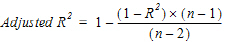
where n is the number of data points in the regression and R2 is the square of the correlation coefficient.
WinNonlin estimates Lambda Z using the regression with the largest adjusted R2 and:
•If the adjusted R2 does not improve, but is within 0.0001 of the largest adjusted R2 value, the regression with the larger number of points is used.
•Lambda Z must be calculated from at least three data points.
•The estimated slope must be negative, so that its negative Lambda Z is positive.
For sparse sampling data: For sparse data, the mean concentration at each time (plasma or serum data) or mean rate for each interval (urine data) is used when estimating Lambda Z. Otherwise, the method is the same as for concentration data.
For drug effect data: Phoenix will compute the best-fitting slopes at the beginning of the data and at the end of the data using the same rules that are used for Lambda Z (best adjusted R-square with at least three points), with the exception that linear or log regression can be used according to the user's choice and the estimated slope can be positive or negative. If the user specifies the range only for Slope1, then in addition to computing Slope1, WinNonlin will compute the best-fitting slope at the end of the data for Slope2. If the user specifies the range only for Slope2, then WinNonlin will also compute the best-fitting slope at the beginning of the data for Slope1.
The data points included in each slope are indicated on the Summary table of the output workbook and text for model 220. Data points for Slope1 are marked with “1” in workbook output and footnoted using “#” in text output; data points for Slope2 are labeled “2” and footnoted using an asterisk, “*”.
Calculation of Lambda Z
Once the time points being used in the regression have been determined either from the Best Fit method or from the user’s specified time range, Phoenix can estimate Lambda Z by performing a regression of the natural logarithm of the concentration values in this range of sampling times. The estimate slope must be negative, Lambda Z is defined as the negative of the estimated slope.
Note:Using this methodology, Phoenix will almost always compute an estimate for Lambda Z. It is the user’s responsibility to evaluate the appropriateness of the estimated value.
Calculation of slopes for effect data
Phoenix estimates slopes by performing a regression of the response values or their natural logarithm depending on the user’s selection. The actual slopes are reported; they are not negated as for Lambda Z.
Limitations of Lambda Z and slope estimation
It is not possible for Phoenix to estimate Lambda Z or slope in the following cases.
•There are only two non-missing observations and the user requested automatic range selection (Best Fit).
•The user-specified range contains fewer than two non-missing observations.
•Automatic range selection is chosen, but there are fewer than three positive concentration values after the Cmax of the profile for non-bolus models and fewer than two for bolus models or the slope is not negative.
•For infusion data, automatic range selection is chosen, and there are fewer than three points at or after the infusion stop time.
•The time difference between the first and last data points in the estimation range used is approximately < 1e –10.
In these instances, the curve fit for that subject will be omitted. The parameters that do not depend on Lambda Z (i.e., Cmax, Tmax, AUClast, etc.) will still be reported, but the software will issue a warning in the text output, indicating that Lambda Z was not estimable.
For non-compartmental analysis of concentration data, Phoenix computes additional parameters listed in the table below. The parameters included depend on whether upper, lower, or both limits are supplied. See “Therapeutic response windows” for additional computation details.
|
Time Range for Computation |
Parameter |
Description |
Parameter Reported? |
|
|
Conc Limits Specified |
||||
|
Lower only |
Lower+Upper |
|||
|
Dose time to last observation |
TimeLow |
Total time below lower limit |
Yes |
Yes |
|
TimeBetween |
Total time between lower/upper limits |
No |
Yes |
|
|
TimeHigh |
Total time above upper limit |
Yes |
Yes |
|
|
AUCLow |
AUC that falls below lower limit |
Yes |
Yes |
|
|
AUCBetween |
AUC that falls between lower/upper limits |
No |
Yes |
|
|
AUCHigh |
AUC that falls above upper limit |
Yes |
Yes |
|
|
Dose time to infinity using Lambda Z (if Lambda Z exists) |
TimeInfBetween |
Total time (extrapolated to infinity) between lower/upper limits |
No |
Yes |
|
TimeInfHigh |
Total time (extrapolated to infinity) above upper limit |
Yes |
Yes |
|
|
AUCInfLow |
AUC (extrapolated to infinity) that falls below lower limit |
Yes |
Yes |
|
|
AUCInfBetween |
AUC (extrapolated to infinity) that falls between lower/upper limits |
No |
Yes |
|
|
AUCInfHigh |
AUC (extrapolated to infinity) that falls above upper limit |
Yes |
Yes |
|
For therapeutic windows, one or two boundaries for concentration values can be given, and the program computes the time spent in each window determined by the boundaries and computes the area under the curve contained in each window. To compute these values, for each pair of consecutive data points, including the inserted point at dosing time if there is one, it is determined if a boundary crossing occurred in that interval. Call the pair of time values from the dataset (ti, ti+1) and called the boundaries ylower and yupper.
If no boundary crossing occurred, the difference ti+1, ti is added to the appropriate parameter TimeLow, TimeBetween, or TimeHigh, depending on which window the concentration values are in. The AUC for (ti, ti+1) is computed following the user’s specified AUC calculation method as described in the section on the “Options tab”. Call this AUC*. The parts of this AUC* are added to the appropriate parameters AUCLow, AUCBetween, or AUCHigh. For example, if the concentration values for this interval occur above the upper boundary, the rectangle that is under the lower boundary is added to AUCLow, the rectangle that is between the two boundaries is added to AUCBetween and the piece that is left is added to AUCHigh. This is equivalent to these formulae:
|
AUCLow=AUCLow+ylower*(ti+1 – ti) |
(2) |
|
AUCBetween=AUCBetween+(yupper – ylower)*(ti+1 – ti) |
(3) |
|
AUCHigh=AUCHigh+AUC* – yupper*(ti+1 – ti) |
(4) |
If there was one boundary crossing, an interpolation is done to get the time value where the crossing occurred; call this t*. The interpolation is done by either the linear rule or the log rule following the user’s AUC calculation method as described above in section 3, i.e., the same rule is used as when inserting a point for partial areas. To interpolate to get time t* in the interval (ti, ti+1) at which the concentration value is yw:
Linear interpolation rule for time:
|
t*=ti+[(yw – yi)/(yi+1 – yi)]*(ti+1 – ti) |
(5) |
Log interpolation rule for time:
|
t*=ti+[(ln(yw) – ln(yi))/(ln(yi+1) – ln(yi))]*(ti+1 – ti) |
(6) |
The AUC for (ti, t*) is computed following the user’s specified AUC calculation method. The difference t* – ti is added to the appropriate time parameter and the parts of the AUC are added to the appropriate AUC parameters. Then the process is repeated for the interval (t*, ti+1).
If there were two boundary crossings, an interpolation is done to get t* as above for the first boundary crossing, and the time and parts of AUC are added in for the interval (ti, t*) as above. Then another interpolation is done from ti to ti+1 to get the time of the second crossing t** between (t*, ti+1), and the time and parts of AUC are added in for the interval (t*, t**). Then the times and parts of AUC are added in for the interval (t**, ti+1).
The extrapolated times and areas after the last data point are now considered for the therapeutic window parameters that are extrapolated to infinity. For any of the AUC calculation methods, the AUC rule after tlast is the log rule, unless an endpoint for the interval is negative or zero in which case the linear rule must be used. The extrapolation rule for finding the time t* at which the extrapolated curve would cross the boundary concentration yw is:
|
t*=(1/Lambda_z)*(Lambda_z_intercept – ln(yw)) |
(7) |
If the last concentration value in the dataset is zero, the zero value was used in the above computation for the last interval, but now ylast is replaced with the following if Lambda Z is estimable:
|
ylast=exp(Lambda_z_intercept – Lambda_z*tlast) |
(8) |
If ylast is in the lower window: InfBetween and InfHigh values are the same as Between and High values. If Lambda Z is not estimable, AUCInfLow is missing. Otherwise:
|
AUCInfLow=AUCLow+ylast/Lambda_z |
(9) |
If ylast is in the middle window for two boundaries: InfHigh values are the same as High values. If Lambda Z is not estimable, InfLow and InfBetween parameters are missing. Otherwise: Use the extrapolation rule to get t* at the lower boundary concentration. Add time from tlast to t* into TimeInfBetween. Compute AUC* from tlast to t*, add the rectangle that is under the lower boundary into AUCInfLow, and add the piece that is left into AUCInfBetween. Add the extrapolated area in the lower window into AUCInfLow. This is equivalent to:
|
t*=(1/Lambda_z)*(Lambda_z_intercept – ln(ylower)) |
(10) |
|
TimeInfBetween=TimeBetween+(t* – tlast) |
(11) |
|
AUCInfBetween=AUCBetween+AUC* – ylower*(t* – tlast) |
(12) |
|
AUCInfLow=AUCLow+ylower*(t* – tlast)+ylower/Lambda_z |
(13) |
If ylast is in the top window when only one boundary is given, the above procedure is followed and the InfBetween parameters become the InfHigh parameters.
If there are two boundaries and ylast is in the top window: If Lambda Z is not estimable, all extrapolated parameters are missing. Otherwise, use the extrapolation rule to get t* at the upper boundary concentration value. Add time from tlast to t* into TimeInfHigh. Compute AUC* for tlast to t*, add the rectangle that is under the lower boundary into AUCInfLow, add the rectangle that is in the middle window into AUCInfBetween, and add the piece that is left into AUCInfHigh. Use the extrapolation rule to get t** at the lower boundary concentration value. Add time from t* to t** into TimeInfBetween. Compute AUC** from t* to t**, add the rectangle that is under the lower boundary into AUCInfLow, and add the piece that is left into AUCInfBetween. Add the extrapolated area in the lower window into AUCInfLow. This is equivalent to:
|
t*=(1/Lambda_z)*(Lambda_z_intercept – ln(yupper)) |
(14) |
|
t**=(1/Lambda_z)*(Lambda_z_intercept – ln(ylower)) |
(15) |
|
TimeInfHigh=TimeHigh+(t* – tlast) |
(16) |
|
TimeInfBetween=TimeBetween+(t** – t*) |
(17) |
|
AUCInfHigh=AUCHigh+AUC* – yupper*(t* – tlast) |
(18) |
|
AUCInfBetween=AUCBetween+(yupper – ylower)*(t* – tlast)+AUC** – ylower*(t** – t*) |
(19) |
|
AUCInfLow=AUCLow+ylower*(t* – tlast)+ylower*(t** – t*)+ylower/Lambda_z |
(20) |
|
|
(21) |
|
|
(22) |
|
|
(23) |
|
|
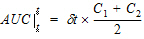
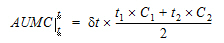
(24) |
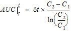
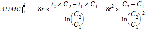
where dt is (t2 – t1).
Note:If the logarithmic trapezoidal rule fails in an interval because C1 <= 0, C2 <= 0, or C1=C2, then the linear trapezoidal rule will apply for that interval.
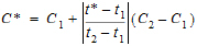
Linear interpolation rule (to find C* at time t* for t1 < t* < t2)
|
|
(25) |
Logarithmic interpolation rule
|
|
(26) |
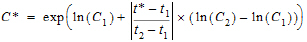
Note:If the logarithmic interpolation rule fails in an interval because C1 <= 0 or C2 <= 0, then the linear interpolation rule will apply for that interval.
Extrapolation (to find C* after the last numeric observation)
Additional rules for plasma and urine models
The following additional rules apply for plasma and urine models (not model 220 for Drug Effect):
-
If a start or end time falls before the first observation and after the dose time, the corresponding Y value is interpolated between the first data point and C0. C0=0 except in IV bolus models (model 201), where C0 is the dosing time intercept estimated by Phoenix, and except for models 200 and 202 at steady state, where C0 is the minimum value between dose time and tau.
-
If a start or end time falls within the range of the data but does not coincide with an observed data point, then a linear or logarithmic interpolation is done to estimate the corresponding Y, according to the AUC Calculation method selected in the NCA Options. (See “Options tab”.) Note that logarithmic interpolation is overridden by linear interpolation in the case of a non-positive endpoint.
-
If a start or end time occurs after the last numeric observation (i.e., not “missing” or “BQL”) and Lambda Z is estimable, Lambda Z is used to estimate the corresponding Y:
|
Y=exp(Lambda_z_intercept – Lambda_z*t) |
(27) |
The values Lambda_z_intercept and Lambda Z are those values found during the regression for Lambda Z. Note that a last observation of zero will be used for linear interpolation, i.e., this rule does not apply prior to a last observation of zero.
-
If a start or end time falls after the last numeric observation and Lambda Z is not estimable, the partial area will not be calculated.
-
If both the start and end time for a partial area fall at or after the last positive observation, then the log trapezoidal rule will be used. However, if any intervals used in computing the partial area have non-positive endpoints or equal endpoints (for example, there is an observation of zero that is used in computing the partial area), then the linear trapezoidal rule will override the log trapezoidal rule.
-
If the start time for a partial area is before the last numeric observation and the end time is after the last numeric observation, then the log trapezoidal rule will be used for the area from the last observation time to the end time of the partial area. However, if the last observation is non-positive or is equal to the extrapolated value for the end time of the partial area, then the linear trapezoidal rule will override the log trapezoidal rule.
The end time for the partial area must be greater than the start time. Both the start and end time for the partial area must be at or after the dosing time.
The NCA object provides special methods to analyze concentration data with few observations per subject. The NCA object treats this sparse data as a special case of plasma or urine concentration data. It first calculates the mean concentration curve of the data, by taking the mean concentration value for each unique time value for plasma data, or the mean rate value for each unique midpoint for urine data. For this reason, it is recommended to use nominal time, rather than actual time, for these analyses. The standard error of the data is also calculated for each unique time or midpoint value.
Using the mean concentration curve, the NCA object calculates all of the usual plasma or urine final parameters listed under “NCA parameter formulas”. In addition, it uses the subject information to calculate standard errors that will account for any correlations in the data resulting from repeated sampling of individual animals.
The NCA sparse methodology calculates PK parameters based on the mean profile for all the subjects in the dataset. For batch designs, where multiple time points are measured for each subject, this methodology only generates unbiased estimates if equal sample sizes per time point are present. If this is not the case, then bias in the parameter estimates is introduced.
Note:In order to create unbiased estimates, the sparse sampling routines used in the NCA object require that the dataset does not contain missing data.
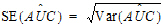
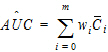
For plasma data (models 200–202), the NCA object calculates the standard error for the mean concentration curve’s maximum value (Cmax), and for the area under the mean concentration curve from dose time through the final observed time (AUCall). Standard error of the mean Cmax will be calculated as the sample standard deviation of the y-values at time Tmax divided by the square root of the number of observations at Tmax, or equivalently, the sample standard error of the y-values at Tmax. Standard error of the mean AUC will be calculated as described in Nedelman and Jia (1998), using a modification in Holder (2001), and will account for any correlations in the data resulting from repeated sampling of individual animals. Specifically:
|
|
(28) |
Since AUC is calculated by the linear trapezoidal rule as a linear combination of the mean concentration values,
|
|
(29) |
where:
•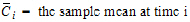
•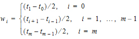
•m=last observation time for AUCall, or time of last measurable (positive) mean concentration for AUClast
it follows that:
|
|
(30) |
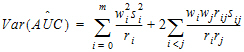
where:
•
•
•
• for
for
all animals k that are sampled at both times i and j.
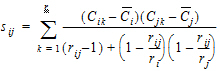
The above equations can be computed from basic statistics, and appear as equation (7.vii) in Nedelman and Jia (1998). When computing the sample covariances in the above, NCA uses the unbiased sample covariance estimator, which can be found as equation (A3) in Holder (2001):
|
|
(31) |
For urine models (models 210–212), the standard errors are computed for Max_Rate, the maximum observed excretion rate, and for AURC_all, the area under the mean rate curve through the final observed rate.
For cases where a non-zero value C0 must be inserted at dose time t0 to obtain better AUC estimates (see “Data checking and pre-treatment”), the AUC estimate contains an additional constant term: C*=C0(t1 – t0)/2. In other words, w0 is multiplied by C0, instead of being multiplied by zero as occurs when the point (0,0) is inserted. An added constant in AÛC will not change Var(AÛC), so SE_AUClast and SE_AUCall also will not change. Note that the inserted C0 is treated as a constant even when it must be estimated from other points in the dataset, so that the variances and covariances of those other data points are not duplicated in the Var(AÛC) computation.
For the case in which rij=1, and ri=1 or rj=1, then sij is set to 0 (zero).
The AUCs must be calculated using one of the linear trapezoidal rules. Select a rule using the instructions listed under “Options tab”.
NCA for drug effect data requires the following input data variables:
•Dependent variable, i.e., response or effect values (continuous scale)
•Independent variable, generally the time of each observation. For non-time-based data, such as concentration-effect data, take care to interpret output parameters such as “Tmin” (independent variable value corresponding to minimum dependent variable value) accordingly.
It also requires the following constants:
•Dose time (relative to observation times), entered in the Dosing worksheet
•Baseline response value, entered in the Therapeutic Response tab of the Model Properties or pulled from a Dosing worksheet as described below
•Threshold response value (optional), entered in the Therapeutic Response tab of the NCA Diagram
If the user does not enter a baseline response value, the baseline is assumed to be zero, with the following exception. When working from a Certara Integral study that includes a Dosing worksheet, if no baseline is provided by the user, Phoenix will use the response value at dose time as baseline, and if the dataset does not include a response at dose time, the user will be required to supply the baseline value.
If there is no response value at dose time, or if dose time is not given, see “Data checking and pre-treatment” for the insertion of the point (dosetime, baseline).
Instead of Lambda Z calculations, as computed in NCA PK models, the NCA PD model can calculate the slope of the time-effect curve for specific data ranges in each profile. Unlike Lambda Z, these slopes are reported as their actual value rather than their negative. See “Lambda Z or Slope Estimation settings” for more information.
Like other NCA models, the PD model can compute partial areas under the curve, but only within the range of the data (no extrapolation is done). If a start or end time does not coincide with an observed data point, then interpolation is done to estimate the corresponding Y, following the equations and rules described under “Partial area calculation”.
For PD data, the default and recommended method for AUC calculation is the Linear Trapezoidal with Linear Interpolation (set as described under “Options tab”.) Use caution with log trapezoidal since areas are calculated both under the curve and above the curve. If the log trapezoidal rule is appropriate for the area under a curve, then it would underestimate the area over the curve. For this reason, Phoenix uses the linear trapezoidal rule for area where the curve is below baseline when computing AUC_Below_B, and similarly for threshold and AUC_Below_T.
Phoenix provides flexibility in performing weighted nonlinear regression and using weighted regression. Weights are assigned using menu options or by adding weighting values to a dataset. Each operational object in Phoenix that uses weighted values has instructions for using weighting.
There are three ways to assign weights, other than uniform weighting, through the Phoenix user interface:
•Weighted least squares: weight by a power of the observed value of Y.
•Iterative reweighting: weight by a power of the predicted value of Y.
•Reading weights from the dataset: include weight as a column in the dataset.
When using weighted least squares, Phoenix weights each observation by the value of the dependent variable raised to the power of n. That is, WEIGHT=Yn. For example, selecting this option and setting n= –0.5 instructs Phoenix to weight the data by the square root of the reciprocal of observed Y:
|
|
(32) |

If n has a negative value, and one or more of the Y values are less than or equal to zero, then the corresponding weights are set to zero.
The application scales the weights such that the sum of the weights for each function equals the number of observations with non-zero weights. See “Scaling of weights”.
Iterative Reweighting redefines the weights for each observation to be Fn, where F is the predicted response. For example, selecting this option and setting n= –0.5 instructs Phoenix to weight the data by the square root of reciprocal of the predicted value of Y, i.e.,
|
|
(33) |

As with Weighted least squares, if N is negative, and one or more of the predicted Y values are less than or equal to zero, then the corresponding weights are set to zero.
Iterative reweighting differs from weighted least squares in that for weighted least squares the weights are fixed. For iteratively re-weighted least squares the parameters change at each iteration, and therefore the predicted values and the weights change at each iteration.
For certain types of models, iterative reweighting can be used to obtain maximum likelihood estimates. For more information see the article by Jennrich and Moore (1975). Maximum likelihood estimation by means of nonlinear least squares. Amer Stat Assoc Proceedings Statistical Computing Section 57–65.
Reading weights from the dataset
It is also possible to have a variable in the dataset that has as its values the weights to use. The weights should be the reciprocal of the variance of the observations. As with Weighted Least Squares, the application scales the weights such that the sum of the weights for each function equals the number of observations with non-zero weights.
When weights are read from a dataset or when weighted least squares is used, the weights for the individual data values are scaled so that the sum of the weights for each function is equal to the number of data values with non-zero weights.
The scaling of the weights has no effect on the model fitting as the weights of the observations are proportionally the same. However, scaling of the weights provides increased numerical stability.
Consider the following example:
|
X |
Y |
Y–2 |
Weight assigned by Phoenix |
|
1 |
6 |
0.0278 |
1.843 |
|
10 |
9 |
0.0123 |
0.819 |
|
100 |
14 |
0.0051 |
0.338 |
|
Sum |
|
0.0452 |
3.000 |
Suppose weighted least squares with the power –2 was specified, which is the same as weighting by 1/Y*Y. The corresponding values are as shown in the third column. Each value of Y–2 is divided by the sum of the values in the third column, and then multiplied by the number of observations, so that:
(0.0277778/.0452254)*3=1.8426238, or 1.843 after rounding.
Note that 0.0278/0.0051 is the same proportion as 1.843/0.338.
