Review of Laplacian-Approximation Formulation

For nonlinear mixed-effect models, there are usually two levels of variability:

intra-individual variability due to residual/measurement errors; and

inter-individual variability in parameter values due to “unexplained” variation (e.g., natural, biological variation) and/or covariates.

For example, an observable variable may be governed by the statistical model:

where

is the j^th observation (e.g., drug concentration) for subject i at time .

f is the function relating time , parameter specific to subject i, and parameter common to all subjects to observation .

is a random vector to account for the inter-individual variability

is often referred to as bare fixed effects as they are not paired with any random effects

is the residual error at for subject i, where the functional form of r determines the type of residual error (e.g., if r ≡ 1, then it is an additive error; and if r ≡ f, then it is a proportional/multiplicative error) and random variables () are assumed to be independent and identically (i.i.d.) normally distributed with zero mean and constant variance ².

m_i is the number of observations for subject i.

N_SUB is the number of subjects.

Most PKPD population analysis are based on parametric assumptions, where the distribution of is assumed to be i.i.d. multivariate normally distributed. (Note that the distribution can also be the transformations of multivariate normal distribution.) Specifically, it is assumed that , where and is independent and identically multi-normally distributed with zero mean and covariance matrix ; that is, with .

It is also assumed that and are independent. The goal of parametric methods is to find the estimates for population parameters, , , , and with given data. Most derivations in this section are based on work reported in reference [1].

Let . Then, due to the i.i.d. normal assumption on , the conditional PDF of given is given by

Since 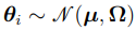, the PDF of is given by

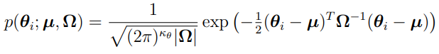
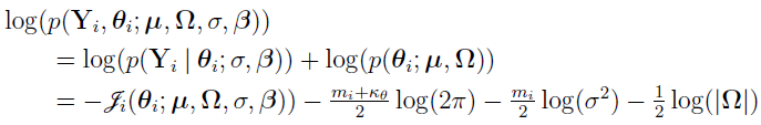
Thus the logarithm of the joint PDF of and is given by

where

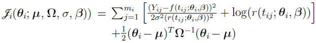
With given, , , , and , one can optimize to obtain optimal individual parameter estimates for the i^th individual, i = 1, 2,..., N_SUB. These estimates are also referred to as conditional modes, modes of a posterior (MAP), empirical Bayes estimates (EBE) or posthoc. This is the method used to calculate individual parameter estimates for all the population analysis methods except for the EM method, which uses the conditional means rather than modes.

   The marginal PDF of is given by . Note that is independent (due to the independence of ). Hence, the marginal PDF of () is given by

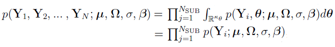
which implies that .

The goal of maximum likelihood methods is to maximize overall log-likelihood function (as shown in the previous equation) to obtain estimates for population parameters. Unfortunately, the marginal PDF often cannot be computed analytically due to the complexity of the involved integral. There are two main methods to solve this problem.

Approximate the required integral (e.g., through linearization, Laplacian approximation, or Gaussian quadrature method) and then maximize the resulting approximate marginal PDF to obtain population parameter estimates. The unconstrained Broyden–Fletcher–Goldfarb–Shanno (BFGS) quasi-Newton method is then often used for the corresponding optimization problem. This is the optimization algorithm used by Certara’s NLME engine.

Use the EM method, which alternates between an expectation step and a maximization step to obtain the parameter estimates that potentially will iteratively converge to the maximum likelihood estimates (refer to the “Expectation Maximization-Based Algorithms” for more information).

It is worth noting that, since is a symmetric matrix, instead of estimating directly, one often estimates its corresponding lower triangular matrix (that is, 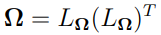with obtained by using Cholesky decomposition). This is the method used in Certara’s NLME engine.

Before further exploration of the Laplacian-approximation-based algorithms, some additional notations should be defined. Let 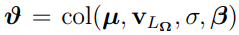, where col is an operator that transforms a sequence of column vectors into a single column vector by stacking them one under the other. Then 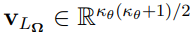is obtained by eliminating the above diagonal elements of .

.

Legal Notice | Contact Certara
© Certara USA, Inc. All rights reserved.