Linearization Method and the Resulting Algorithms
The linearization method involves linearization of f in  (discussed in “Review of Laplacian-Approximation Formulation”) around
  and then replacing
  with
with  . Two values are often chosen for the linearization point
  :
:
 (that is,
  = 0), i = 1, 2,..., NSUB
The resulting algorithm is the first-order (FO) method.
![]() ,the conditional modes obtained using the current population parameter estimates, i = 1, 2,..., NSUB.
,the conditional modes obtained using the current population parameter estimates, i = 1, 2,..., NSUB.
The resulting algorithm is the first-order conditional estimation method (FOCE method).
For the linearization method,  is approximated as
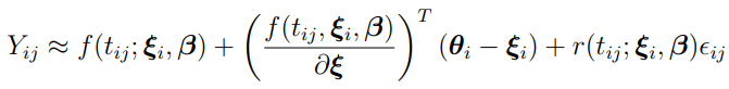
for j = 1, 2,..., mi, i = 1, 2,..., NSUB.
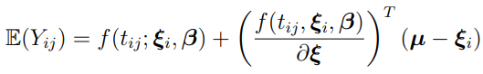
Due to the normal and independent assumptions on  and
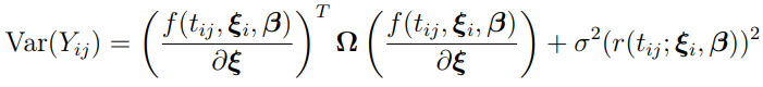
and  , is approximately normally distributed with mean and variance, respectively given by
and
Thus, the logarithm of the marginal PDF is approximated as

where

Note that the approximate marginal PDF obtained above depends on the assumption that is i.i.d. normally distributed. Hence, the linearization methods are only applicable to normal/Gaussian data.
For simple problems, the linearization method is usually faster than the other approximation methods, and the estimates are usually accurate. However, if the model is highly nonlinear, then the linearization method may provide a poor approximation to the marginal PDF, and hence the estimates obtained may be far less accurate.