Sometimes it is desirable to see the mean response for each level of a classification variable or for each combination of levels for two or more classification variables. If there are covariables with unequal means for the different levels, or if there are unbalanced data, the subsample means are not estimates that can be validly compared. This section describes least squares means, statistics that make proper adjustments for unequal covariable means and unbalanced data in the linear mixed effects model.
Consider a completely randomized design with a covariable. The model is:

where yij is the observed response on the jth individual on the ith treatment; ai is the intercept for the ith treatment; xij is the value of the covariable for the jth individual in the ith treatment; b is the slope with respect to x; and eij is a random error with zero expected value. Suppose there are two treatments; the average of the x1j is 5; and the average of the x2j is 15. The respective expected values of the sample means are a1+5b and a2+15b. These are not comparable because of the different coefficients of b. Instead, one can estimate a1+10b and a2+10b where the overall mean of the covariable is used in each linear combination.
Now consider a 2 ´ 2 factorial design. The model is:

where yijk is the observed response on the kth individual on the ith level of factor A and the jth level of factor B; m is the over-all mean; ai is the effect of the ith level of factor A; bj is the effect of the jth level of factor B; and eijk is a random error with zero expected value. Suppose there are six observations for the combinations where i=j and four observations for the combinations where i ¹ j. The respective expected values of the averages of all values on level 1 of A and the averages of all values on level 2 of A are m + (0.6 b1 + 0.4 b2) + a1 and m + (0.4 b1 + 0.6 b2) + a2. Thus, sample means cannot be used to compare levels of A because they contain different functions of b1 and b2. Instead, one compares the linear combinations:

The preceding examples constructed linear combinations of parameters, in the presence of unbalanced data, that represent the expected values of sample means in balanced data. This is the idea behind least squares means. Least squares means are given in the context of a defining term, though the process can be repeated for different defining terms for the same model. The defining term must contain only classification variables and it must be one of the terms in the model. Treatment is the defining term in the first example, and factor A is the defining term in the second example. When a least squares means is requested, LinMix automatically generates the coefficients lj of the linear combination expression and processes them almost as it would process the coefficients specified in an estimate statement. This chapter describes generation of linear combinations of elements of b that represent least squares means. A set of coefficients are created for each of all combinations of levels of the classification variables in the defining term. For all variables in the model, but not in the defining term, average values of the variables are the coefficients. The average value of a numeric variable (covariable) is the average for all cases used in the model fitting. For a classification variable with k levels, assume the average of each indicator variable is 1/k. The value 1/k would be the actual average if the data were balanced. The values of all variables in the model have now been defined. If some terms in the model are products, the products are formed using the same rules used for constructing rows of the X matrix as described in the “Fixed effects specification” section. It is possible that some least squares means are not estimable.
For example, suppose the fixed portion of the model is: Drug + Form + Age + Drug*Form
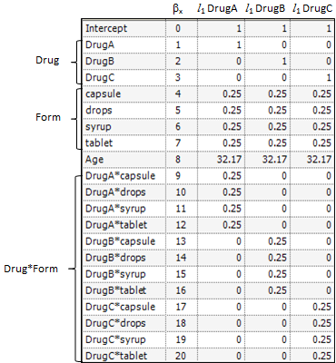
To get means for each level of Drug, the defining term is Drug. Since Drug has three levels, three sets of coefficients are created. Build the coefficients associated the first level of Drug, DrugA. The first coefficient is one for the implied intercept. The next three coefficients are 1, 0, and 0, the indicator variables associated with DrugA. Form is not in the defining term, so average values are used. The next four coefficients are all 0.25, the average of a four factor indicator variable with balanced data. The next coefficient is 32.17, the average of Age. The next twelve elements are:

The final result is shown in the DrugA column in the following table. The results for DrugB and DrugC are also shown in the table. No new principles would be illustrated by finding the coefficients for the Form least squares means. The coefficients for the Drug*Form least squares means would be like representative rows of X except that Age would be replaced by the average of Age.
