Phoenix's noncompartmental analysis (NCA) engine computes derived measurements from raw data by using methods appropriate for either serially- or sparsely-sampled data. Phoenix provides the following NCA models for different types of input data:
aTau is required for steady-state data only.
Models 200–202 can be used for either single-dose or steady-state data. For steady-state data, the computation assumes equal dosing intervals (Tau) for each profile, and that the data are from a “final” dose given at steady-state.
Models 210–212 (urine concentrations) assume single-dose data, and the final parameters do not depend on the dose type.
The plasma and urine models support rich datasets as well as sparsely-sampled studies such as toxicokinetic studies. The drug effect model is for analysis of slope, height, areas, and moments in richly-sampled time-effect data.
Use one of the following to add an NCA object to a Workflow:
Right-click menu for a Workflow object: New > NCA and Toolbox > NCA.
Main menu: Insert > NCA and Toolbox > NCA.
Right-click menu for a worksheet: Send To > NCA and Toolbox > NCA.
Note:To view the object in its own window, select it in the Object Browser and double-click it or press ENTER. All instructions for setting up and execution are the same whether the object is viewed in its own window or in Phoenix view.
This section contains information on the following topics:
Use the Main Mappings panel to identify how a dataset is used with an NCA object by mapping data types in a dataset to the appropriate contexts. Context associations change depending on the selected NCA model. Required input is highlighted orange in the interface.
•None: Data types mapped to this context are not included in any analysis or output.
•Sort: Categorical variable(s) identifying individual data profiles, such as subject ID in an NCA study. A separate analysis is done for each unique combination of sort variable values.
•Carry: Data variable(s) to include in the output worksheets. Note that time-dependent data variables (those that change over the course of a profile) are not carried over to time-independent output (e.g., Final Parameters), only to time-dependent output (e.g., Summary).
Plasma study
•Time: Nominal or actual time collection points in a plasma study.
•Concentration: Drug concentration values in the blood of a plasma study.
(Plasma Models with Sparse Sampling also require a single Subject mapping.)
Urine study
•Start Time: Starting times for individual collection intervals during a urine study.
•End Time: Ending times for individual collection intervals during a urine study.
•Concentration: Dependent variable, drug concentration in urine.
•Volume: Volume of urine collected per time interval.
Drug effect study
•X: Time values for the drug effect data.
•Y: Drug effect or response values.
The Dosing panel allows users to type or map dosing data for the different NCA models.
•Models 200–202 (plasma) assume that data were taken after a single dose or after a final dose at steady state. For steady state Phoenix also assumes equal dosing intervals.
•Models 210–212 (urine) assume single-dose urine data. If dose time is not entered, Phoenix uses a time of zero.
•Model 220 (drug effect) uses the same time scale and units as the input dataset. Users enter the time of the most recent dose for each profile.
The Dosing panel columns change depending on the model type and dose type selected in the Options tab.
The first time a user selects the Dosing panel, if sort keys are defined in the Main Mappings panel, Phoenix displays the Dosing sorts dialog.
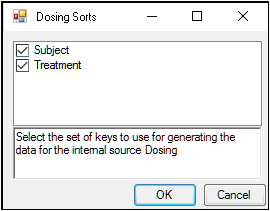
The dialog has all of the currently specified sort variables selected by default. The selected sort variables will be used when creating the internal dosing worksheet. To select a subset of the sort variables, clear the checkbox beside the unwanted variable and click OK.
Context associations change depending on the selected NCA model. Required input is highlighted orange in the interface.
•None: Data types mapped to this context are not included in any analysis or output.
•Sort: Categorical variable(s) identifying individual data profiles. A separate computation is done for each unique combination of sort variable values.
•Time: Time of dose administration.
•Dose: Amount of drug per profile.
•Tau: The (assumed equal) dosing interval for steady-state data. TAU must be a positive number for steady-state profiles and blank for non-steady-state profiles.
•Infusion_Length: Total amount of time for an IV infusion.
•Dose_Type: Dosing route, if not defined in the Options tab.
Note:The time units for the dosing data must be the same as the time units for the time/concentration data.
Phoenix attempts to estimate the rate constant, Lambda Z, associated with the terminal elimination phase for concentration data. If Lambda Z is estimable, parameters for concentration data will be extrapolated to infinity. For drug effect models, Phoenix estimates the two slopes at the beginning and end of the data. NCA does not extrapolate beyond the observed data for drug effect models.
The observed times for each profile are displayed in a graph on separate tabs in the Slopes Selector panel. Below are usage instructions. For descriptions of how the NCA object determines Lambda Z or slope estimation settings, see “Lambda Z or Slope Estimation settings”.
Note:Any changes to the settings available in the Slopes Selector panel also affect the Slopes panel and vice versa.
-
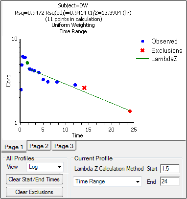
Use the View menu to select a linear (Lin) or logarithmic (Log) axis scale.
-
Use the Lambda Z Calculation Method menu to select a method.
If Best Fit is selected, Phoenix calculates the points for Lambda Z estimation for each profile.
If Time Range is selected, users must enter the start and end times for Lambda Z estimation. -
To turn off Lambda Z or slope estimation for all profiles, select the Disable Curve Stripping checkbox in the Options tab. For more information see step 4 in “Model settings”.
Users can manually select start times, end times, and excluded time points by selecting them on the graph for each profile (this action automatically sets the Lambda Z Calculation Method to Time Range.
•Click a data point on a graph to select the start time.
•SHIFT+click a data point on a graph to select the end time.
•CTRL+click a data point on a graph to exclude the time point.
•Change the start time, end time, and exclusions by selecting new points on the graph using the same key combinations listed above.
When the start time, end time, and exclusions are manually selected, the graph title is updated to show the new R2 calculation, the graph is updated to show the new slope, and the legend is updated to show the new slope and exclusions, as shown below.
Note:Excluded data points apply only to Lambda Z or slope calculations. The excluded data points are still included in the computation of AUCs, moments, etc.
Avoid having excluded or zero-valued points at the beginning or end of the Lambda Z range as this can result in inconsistent reporting of the Lambda Z range.For example, if values range from 0.8 to 2 and points before 1.4 are excluded, some of the output reports the range as (0.8, 2), whereas other output lists the range as (1.4, 2).
-
Use the Clear Start/End Times button to have previously selected start time and end time points removed from the graphs in the Slopes Selector panel and from the worksheet in the Slopes panel.
-
Use the Clear Exclusions button to have previously excluded time points included in the graphs in the Slopes Selector panel and in the worksheet in the Slopes panel.
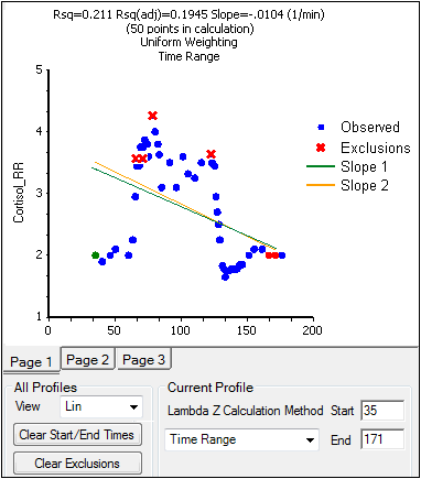
The Drug Effect (220) model calculates two slopes per profile
-
Under Slope Calculation in the Slopes Selector panel, select Slope 1 or Slope 2.
-
Select Linear or Log to set the slope calculation method for slope 1 or slope 2.
-
Use the instructions listed above to select the start times, end times, and exclusions.
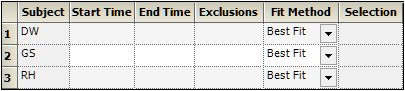
The start time, end time, and exclusions used in the calculation of Lambda Z for each profile are defined in the Slopes panel. Users can type the time points for each profile.
Below are usage instructions. For descriptions of how the NCA object determines Lambda Z or slope estimation settings, see “Lambda Z or Slope Estimation settings”.
Note:Any changes to the settings available in the Slopes panel also affect the Slopes Selector panel and vice versa.
-
Type the start and end time values in the Start Time and End Time columns for each profile.
-
Type excluded time points in the Exclusions column for each profile.
-
Exclude multiple time points for a profile by typing the time points in the same cell and separating the time points with a semicolon.
-
Use the Fit Method menu to specify the method.
If Best Fit is selected, Phoenix calculates the points for Lambda Z estimation.
If Time Range is selected, users must enter the start and end times for Lambda Z estimation. -
To turn off Lambda Z or slope estimation for all profiles, select the Disable Curve Stripping checkbox in the Options tab. For more information see step 4 in “Model settings”.
The Slopes panel for the Drug Effect (220) model also includes options for the slope calculation method.
-
In the Lin/Log column, select Linear or Log to set the slope calculation method.
-
Use the same instructions listed above to select the start times, end times, and exclusions.
The Partial Areas panel includes settings for the computation of partial areas under the curve. Partial area computations are optional. It is not necessary to enter or add any start times or end times in this panel. For descriptions of how the NCA object computes partial areas, see “Partial area calculation”.
•None: Data types mapped to this context are not included in any analysis or output.
•Sort: Categorical variable(s) identifying individual data profiles, such as subject ID in an NCA study. A separate analysis is done for each unique combination of sort variable values.
•Area #: Number to identify the defined partial area.
•Label: Title to use as a label for the defined partial area.
•Start Time: The time at which to begin the partial area calculation.
•End Time: The time at which to end the partial area calculation.
Some additional notes on partial areas:
•Partial area computations are optional. To skip the computations leave the Start Time and End Time columns empty.
•Up to 127 partial areas can be computed per subject.
•The start times and end times can be after the last observed time if Lambda Z is estimable.
The Therapeutic Response panel allows users to determine the time spent within a therapeutic range, and the AUC within the therapeutic range, by using the lower and upper therapeutic response values. For descriptions of how the NCA object handles therapeutic response data, see “Therapeutic response”.
Setting the therapeutic response values is optional for plasma (200–202) and urine (210–212) models. Setting the baseline is recommended for drug effect models (220). The Min Response and Max Response columns show the minimum and maximum concentrations, rates, or responses contained in the datasets.
Caution:When entering or mapping the lower and upper therapeutic ranges of profiles in an NCA urine model, users must enter or map the rate of excretion.
•None: Data types mapped to this context are not included in any analysis or output.
•Sort: Categorical variable(s) identifying individual data profiles, such as subject ID and treatment in a crossover study. A separate analysis is performed for each unique combination of sort variable values.
•Lower (Plasma and Urine study) / Baseline (Drug Effect study): The lower concentration, rate, or response for defining the lower boundary of the target range. This is the lower effect value for each profile. It is required when an external worksheet is mapped. If not specified for the drug effect model, a baseline of zero is used.
•Upper (Plasma and Urine study) / Threshold (Drug Effect): The upper concentration, rate, or response for defining the upper boundary of the target range.
Threshold is the effect value used to calculate additional times and areas. See the “Additional parameters for model 220 with threshold” table.
An NCA object’s display units can be changed to fit a user’s preferences. Each parameter used in a model and the parameter’s default units are listed in the Units panel. Required input is highlighted orange in the interface.
For plasma models (200–202), the time and concentration data must contain units before users can set preferred units.
For plasma models (200–202), the dosing unit must be set before users can set preferred units.
For urine models (210–212), the start time, end time, concentration, and volume data must contain units before users can set preferred units.
For the drug effect model (220), the time and effect data must contain units before users can set preferred units.
•None: Data types mapped to this context are not included in any analysis or output.
•Name: Model parameters associated with the units.
•Default: The model object’s default units.
•Preferred: The user’s preferred units for the parameter.
Note:if you see an “Insufficient units” message, check that units are defined for time and concentration in your input.
Phoenix provides the option to specify the names for NCA model parameters.
•None: (In mapped worksheet only) Rows mapped to this context are not included in any analysis or output.
•Parameter Name: In the internal worksheet, Phoenix’s default parameter names are listed in this column. For a mapped worksheet, click in the cell to indicate that the name in that row is a parameter name.
•Preferred (Name): In the internal worksheet, edit the name that will appear in the output. For a mapped worksheet, click in the cell to indicate that the name in that row is a preferred name.
•Include in Workbook: Indicate whether or not a parameter is included as final parameter in the workbook output.
Note:Parameter names cannot contain empty spaces. The case of each preferred parameter name is preserved.
For more on NCA output parameters see “NCA parameter formulas”.
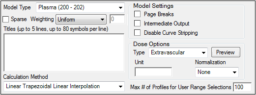
The Options tab allows users to select the NCA model and set options for the selected model.
-
Use the Model Type menu to select the NCA model type (i.e., whether the input data are from plasma, urine, or drug effect measurements). Select Plasma (200-202), Urine (210-212), or Drug Effect (220).
-
Check the Sparse checkbox to use analysis methods for sparse datasets. See “Sparse sampling calculation” for more information on using sparse datasets with NCA models.
-
Use the Weighting menu to select the regression that estimates Lambda Z or slopes. Select User Defined, Uniform, 1/Y, or 1/(Y*Y).
Note:The relative proportions of the weights are important, not the weights themselves. See “Weighting” for more on weighting schemes.
Rules for using the Weighting menu:
•If User Defined is selected then users can enter their own Observed to Power N value. The value of N must be typed in the Weighting text field.
•Sparse data requires Uniform weighting.
•When a log-linear fit is done (Uniform weighting for Lambda Z), then the fit is implicitly using a weighting approximately equal to 1/Yhat2.
Note:If 1/Y and the Linear Log Trapezoidal calculation method are selected, a user might assume that the weighting scheme is 1/LogY, rather than 1/Y. This is not the case, however, since concentrations between zero and one would have negative weights and could not be included in the analysis.
-
Use the Titles text box to type a title for the analysis. The title is displayed at the top of each page in the Core Output and can include up to 5 lines of text.
-
Select a method for calculating the area under the curve from the Calculation Method menu.
The chosen method applies to all AUC, AUMC, and partial area computations. All methods reduce to the log trapezoidal rule, the linear trapezoidal rule, or both. The methods differ based on when the rules are applied. See “Partial area calculation” for descriptive equations of the calculation methods. Select from:
Note:If Sparse Sampling is selected, only linear trapezoidal methods are available.
•Linear Log Trapezoidal. This method uses the linear trapezoidal rule up to Cmax and then the log trapezoidal rule for the remainder of the curve, to compute AUCs. Points for partial areas are inserted using the logarithmic interpolation rule after Cmax, or after C0 for IV bolus, if C0 > Cmax. Otherwise, the linear trapezoidal rule is used. If Cmax is not unique, then the first maximum is used.
•Linear Trapezoidal Linear Interpolation. This is the default method and recommended for Drug Effect Data (220). It uses the linear trapezoidal rule, which is applied to each pair of consecutive points in the dataset that have non-missing values, and sums up these areas to compute AUCs. If a partial area is selected that has an endpoint that is not in the dataset, then the linear interpolation rule is used to insert a concentration value for that endpoint.
•Linear Up Log Down. The linear trapezoidal rule is used to compute AUCs any time that the concentration data is increasing, the logarithmic trapezoidal rule is used any time that the concentration data is decreasing. Points for partial areas are inserted using the linear interpolation rule if the surrounding points show that concentration is increasing, and the logarithmic interpolation rule if the concentration is decreasing.
•Linear Trapezoidal Linear/Log Interpolation. This method is the same as Linear Trapezoidal Linear Interpolation except when a partial area is selected that has an endpoint that is not in the dataset. In that case, the logarithmic interpolation rule is used to insert points after Cmax, or after C0 for IV bolus, if C0 > Cmax. Otherwise, the linear interpolation rule is used. If Cmax is not unique, then the first maximum is used.
Note:The Linear Log Trapezoidal, the Linear Up Log Down, and the Linear Trapezoidal Linear/Log Interpolation methods all apply the same exceptions in area calculation and interpolation. If a Y value (concentration, rate, or effect) is less than or equal to zero, Phoenix defaults to the linear trapezoidal or linear interpolation rule for that point. If adjacent Y values are equal to each other, Phoenix defaults to the linear trapezoidal or linear interpolation rule.
-
Check the Page Breaks checkbox to include page breaks in the ASCII text output.
-
Check the Intermediate Output checkbox to add to the text Core Output the values of each iteration during estimation of Lambda Z and for each of the sub-areas in partial area computations.
-
Check the Disable Curve Stripping checkbox to turn off Lambda Z or slope estimation for all profiles. When this option is selected Lambda Z or slopes are not estimated, parameters that are extrapolated to infinity are not calculated, and the Rules tab is disabled.
-
Disable curve stripping for one or more individual profiles:
•Select Slopes in the Setup tab.
•Enter a start time that is greater than the last time point in a given profile and an end time greater than the start time.
Dose options
Note:Dose Options are not available for the Drug Effect (220) model.
-
Use the Type menu to select the dosing route. Dose type selections determine two things: specific model type and columns available in the Dosing panel. Select Extravascular, IV Bolus, IV Infusion, or Dosing Defined.
-
Set the dosing unit by clicking the Units Builder - Dose
 button or typing the dosing unit into the Unit text field. Only applicable when an internal worksheet is being used for the Dosing data.
See “Using the Units Builder” for more details. -
Click Preview to see a preview of dose option selections in a separate window. Click OK to close the preview window.
-
Use the Normalization menu to select the appropriate factor if the dose amount is normalized by subject body weight or body mass index. Select None, kg. g, mg, m**2, or 1.73 m**2.
•If doses are in milligrams per kilogram of body weight, select mg as the dosing unit and kg as the dose normalization.
•The Normalization menu affects the output parameter units. For example, if dose volume is in liters, selecting kg as the dose normalization changes the units to L/kg.
•Dose normalization affects units for all volume and clearance parameters in NCA models, as well as AUC/D in NCA plasma models, and Percent_Recovered in NCA urine models.
Other options
-
Enter the Max # of Profiles for User Range Selections in the field (default is 100).
If the number of profiles exceeds this value, then the user selection of slopes will be disabled and the engine will calculate the slopes using the Best Fit method. Selecting the Slopes Selector worksheet or Slopes worksheet will display a message notifying the user that the limit has been exceeded and the Best Fit method will be used for all profiles.
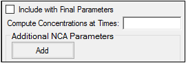
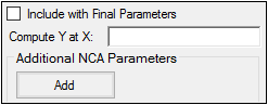
The User Defined Parameters tab allows users to include concentrations/Y values at specified times, as well as additional NCA parameters.
-
Check the Include with Final Parameters box to append the user-defined parameters (both the computed concentrations/Ys and any additional user-defined parameters) to the Final Parameters worksheets, both the pivoted and non-pivoted versions.
-
Enter time or X values at which to compute the concentration or Y value.
•For Plasma models, enter a value(s) in the field to have the NCA object compute the concentration (or the mean concentration, if the Sparse Sampling box in the Options tab is checked) at that time and include the result in the output.
•For Drug Effect models, enter a value(s) in the field to have the NCA object compute the Y value at that X value and include the result in the output.
Up to 30 values can be entered as a comma-separated list. Values can also be specified by using multiple ‘seq’ statements with the format seq(first_time,end_time,increment). For example, seq(0,6,1),8,12,seq(18,36,6).
Note:If a concentration/drug effect value does not exist in the data set for the specified time/X value, it is calculated following the same rules as for computing Y-values for partial area endpoints, see “Partial area calculation”.
-
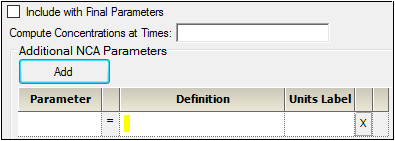
Click Add to define other NCA parameters to include in the output.
-
Enter a name for the parameter in the Parameter column.
The name is checked for validity as it is entered and a message is displayed in the last column of the table if it is not valid. Since the names become column headers in the output, they must also follow the rules for column headers: start with a letter or underscore; contain only letters, numbers, underscores, and ‘%’; and not contain spaces, periods, or symbols. The name cannot match any of the following:
•default names for NCA final parameters
•preferred names for NCA final parameters
•previously defined additional NCA parameters
•names that will be generated by the Compute concentrations at times option
•the words “Dose” and “Sort”
•names of columns defined as Carry variables
-
Enter an equation that defines how the parameter is to be computed in the Definition column. The math function operators +, –, *, /, and ^ can be used in the Definition, as well as ln(x), log(x,base), log10(x), exp(x), and sqrt(x). The parameter can be a function of the following:
•default parameter names (even if selected to be excluded from the results)
•preferred names specified on the Parameter Names setup tab (even if selected to be excluded from the results)
•partial areas
•if an external dosing worksheet is used, the name of the column mapped to Dose and the name of the column mapped to Tau
•if an internal dosing worksheet is used, the “Dose” and “Tau” columns
•Carry variables (names of columns mapped as Carry)
•previously defined user-defined parameter names (those that are above the current name in the user interface)
Note that:
•If more than one dose amount is specified for a profile, the last dose value will be used when computing the parameter.
•If a carryalong is a time-dependent variable (that is, if the carryalong takes on different values per profile), any user-defined parameters defined in terms of this carryalong will be undefined.
•If any of the values to be used when computing the user-defined parameter are missing (for example, an equation that uses Rsq when the Lambda Z fitting fails or was disabled), the value of the user-defined parameter will be missing (blank) in the results.
•Any names used are case-sensitive (they must be correct in terms of uppercase and lowercase).
•To assist with entering final parameter names in the equation, when the user starts to type a name, a dropdown list provides a list of final parameters that match. Double-click an entry from the list to auto-complete typing that name. The list contains only final parameters, even though other names, such as dosing and carryalong names, can be used. The list contains all possible final parameters in NCA, but some may not be applicable to the current selection of model and dosing options.
-
In the Units Label column enter the unit name that is to appear when the parameter values are reported. No conversion of units is done for user-defined parameters.
-
Click the red X in the row to remove that parameter.
The Rules tab contains optional settings that apply to the Lambda Z calculation in Plasma and Urine models. (The Rules tab does not apply to Slope1 and Slope2 in Drug Effect models.)
Rules tab for NCA object
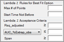
Lambda Z Rules for Best Fit method: These optional rules are used only in the automatic selection of Lambda Z.
•In the Max # of points field, specify the maximum number of points that can be used in the best-fit method for Lambda Z. If a value is specified, the NCA engine will not consider time ranges that contain more than the specified number of points when finding the best Lambda Z. The entered value must be at least 3.
•In the Start Time Not Before field, specify the minimum start time that can be used in the best-fit method for Lambda Z. If a value is specified, the NCA engine will not consider time ranges that start before this minimum start time when finding the best Lambda Z.
Lambda Z Acceptance Criteria: These optional acceptance criteria apply to both the Best Fit method and the Time Range method. These rules are used to flag profiles (described further below) where the Lambda Z final parameter does not meet the specified acceptance criteria.
•Specify the minimum value of Rsq_adjusted that indicates an acceptable fit for Lambda Z in the Rsq_adjusted field. Value must be between 0 and 1.
•Use the pull-down menu to select whether to use AUC_%Extrap_obs or AUC_%Extrap_pred (or, for Urine models, AURC_%Extrap_obs or AURC_%Extrap_pred) when indicating the acceptable fit for Lambda Z. In the field, enter the maximum value to use. Value must be between 0 and 100.
•In the Span field, specify the minimum span or number of half-lives needed for the Lambda Z range to be acceptable. Values must be positive.
If a profile does not have an acceptable Lambda Z fit as specified by the acceptance criteria, an output flag value of ‘Not_Accepted’ is used to flag each of the criterion that is not met by that profile. In addition, a flag value of ‘Missing’ is used to flag all profiles where the parameter used for acceptance cannot be computed. Note that all computed results for flagged profiles are still included in the output, but the final parameters for these profiles will be marked by the flags. All profiles that have an acceptable Lambda Z fit (i.e., meet the acceptance criterion) will have the flag value of ‘Accepted’.
The flags appear in columns in the Final Parameters Pivoted output worksheet immediately after the column for the parameter used for the acceptance criterion. The flag column names are ‘Flag’ appended with the parameter name used for acceptance, e.g., Flag_Rsq_adjusted, Flag_Span. If the user wants to remove the profiles failing to meet the acceptance criteria from the output, the Final Parameters Pivoted worksheet can be processed by the Data Wizard to delete these profiles, by filtering on the flag values of ‘Not_Accepted’ and excluding these rows. Note that the Flag columns do not appear in the output when there are no flagged profiles, that is, when all profiles meet the acceptance criterion or when the acceptance criterion is not set.
In the Final Parameters output worksheet and in the Core Output text, where the final parameter output is stacked, the flag names and values appear below the acceptance parameter. If the acceptance parameter is selected to not be included in the worksheet output in the “Parameters Names” setup, the corresponding flag will also not be included in the worksheet.
See “Data checking and pre-treatment” for a list of cases that also produce flagged output.
The Plots tab allows users to select individual plots to include in the output.
-
Use the checkboxes to toggle the creation of graphs.
-
Click Reset Existing Plots to clear all existing plot output.
Each plot in the Results tab is a single plot object. Every time a model is executed, each object remains the same, but the values used to create the plot are updated. This way, any styles that are applied to the plots are retained no matter how many times the model is executed. Clicking Reset Existing Plots removes the plot objects from the Results tab, which clears any custom changes made to the plot display. -
Use the Enable All and Disable All buttons to check or clear all checkboxes for all plots in the list.
