General linear mixed effects model
Phoenix’s Linear Mixed Effects object is based on the general linear mixed effects model, which can be represented in matrix notation as:
y = Xb + Zg + e
where:
X is the matrix of known constants and the design matrix for b
b is the vector of unknown (fixed effect) parameters
g is the random unobserved vector (the vector of random-effects parameters), normally distributed with mean zero and variance G
Z is the matrix of known constants, the design matrix for g
e is the random vector, normally distributed with mean zero and variance R
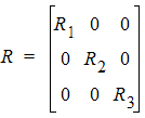
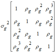
g and e are uncorrelated. In the Linear Mixed Effects object, the Fixed Effects tab is used to specify the model terms for constructing X; the Random tabs in the Variance Structure tab specifies the model terms for constructing Z and the structure of G; and the Repeated tab specifies the structure of R.
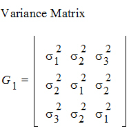
In the linear mixed effects model, if R=s2I and Z=0, then the LinMix model reduces to the ANOVA model. Using the assumptions for the linear mixed effects model, one can show that the variance of y is: V = ZGZT + R.
If Z does not equal zero, i.e., the model includes one or more random effects, the G matrix is determined by the variance structures specified for the random models. If the model includes a repeated specification, then the R matrix is determined by the variance structure specified for the repeated model. If the model doesn’t include a repeated specification, then R is the residual variance, that is R = s2I.
It is instructive to see how a specific example fits into this framework. The fixed effects model is shown in the “Linear mixed effects scenario” section. Listing all the parameters in a vector, one obtains: bT – [m,p1,p2,d1,d2,t1,t2]
For each element of b, there is a corresponding column in the X matrix. In this mode, the X matrix is composed entirely of ones and zeros. The exact method of constructing it is discussed under “Construction of the X matrix”, below.
For each subject, there is one Sk(j). The collection can be directly entered into g. The Z matrix will consist of ones and zeros. Element (i, j) will be one when observation i is from subject j, and zero otherwise. The variance of g is of the form

where Ib represents a b´b identity matrix.
The parameter to be estimated for G is Var{Sk(j)}. The residual variance is:
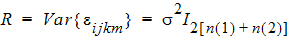
The parameter to be estimated for R is s2.
A summary of the option tabs and the part of the model they generate follows.
Fixed Effects tab specifies the X matrix and generates b.
Variance Structure tab specifies the Z matrix
The Random sub-tab(s) generates G = var(g).
The Repeated tab generates R=var(e).
Additional information is available on the following topics regarding the linear mixed effects general model:
A term is a variable or a product of variables. A user specifies a model by giving a sum of terms. For example, if A and B are variables in the dataset: A + B + AB.
Linear Mixed Effects takes this sum of terms and constructs the X matrix. The way this is done depends upon the nature of the variables A and B.
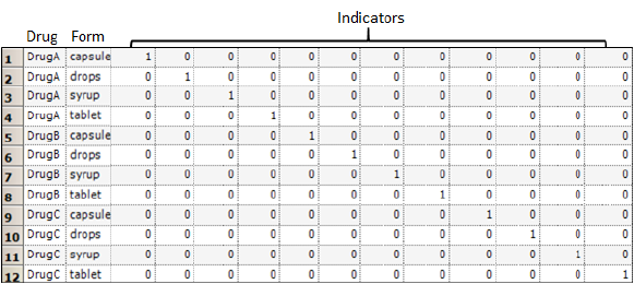
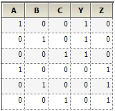
By default, the first column of X contains all ones. The LinMix object references this column as the intercept. To exclude it, select the No Intercept checkbox in the Fixed Effects tab. The rules for translating terms to columns of the X matrix depend on the variable types, regressor/covariate or classification. This is demonstrated using two classification variables, Drug and Form, and two continuous variables, Age and Weight, the “Indicator variables and product of classification with continuous variables” table. A term containing one continuous variable produces a single column in the X matrix.
An integer value is associated with every level of a classification variable. The association between levels and codes is determined by the numerical order for converted numerical variables and by the character collating sequence for converted character variables. When a single classification variable is specified for a model, an indicator variable is placed in the X matrix for each level of the variable. The “Indicator variables and product of classification with continuous variables” table demonstrates this for the variable Drug.
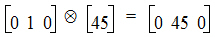
The model specification allows products of variables. The product of two continuous variables is the ordinary product within rows. The product of a classification variable with a continuous variable is obtained by multiplying the continuous value by each column of the indicator variables in each row. For example, the “Indicator variables and product of classification with continuous variables” table shows the product of Drug and Age. The “Two classification plus indicator variables” table shows two classification and indicator variables. The “Product of two classification variables” table gives their product.
The product operations described in the preceding paragraph can be succinctly defined using the Kronecker product. Let A=(aij) be a m´n matrix and let B=(bij) be a p´q matrix. Then the Kronecker product A Ä B=(aij B) is an mp ´ nq matrix expressible as a partitioned matrix with aij B as the (i, j)th partition, i=1,…, m and j=1,…,n.
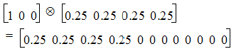
For example, consider the fifth row of the “Indicator variables and product of classification with continuous variables” table. The product of Drug and Age is:
Now consider the fifth row of the “Two classification plus indicator variables” table. The product of Drug and Form is:

The result is the fifth row of the “Product of two classification variables” table.
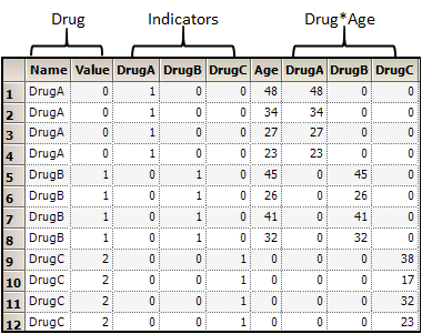
Indicator variables and product of classification with continuous variables
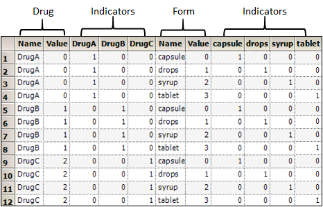
Two classification plus indicator variables
Product of two classification variables
Linear combinations of elements of beta
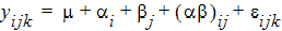
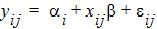
Most of the inference done by LinMix is done with respect to linear combinations of elements of b. Consider, as an example, the model where the expected value of the response of the jth subject on the ith treatment is:
m + ti
where m is a common parameter and m + ti is the expected value of the ith treatment.
Suppose there are three treatments. The X matrix has a column of ones in the first position followed by three treatment indicators.
The b vector is: b = [b0 b1 b2 b3] = [m t1 t2 t3]
The first form is for the general representation of a model. The second form is specific to the model equation shown at the beginning of this section. The expression:

with the lj constant, is called a linear combination of the elements of b.
The range of the subscript j starts with zero if the intercept is in the model and starts with one otherwise. Most common functions of the parameters, such as m+t1, t1 – t3, and t2, can be generated by choosing appropriate values of lj. Linear combinations of b are entered in LinMix through the Estimates and Contrasts tabs. A linear combination of b is said to be estimable if it can be expressed as a linear combination of expected responses. In the context of the model equation (shown at the beginning of this section), a linear combination of the elements of b is estimable if it can be generated by choosing c1, c2, and c3.
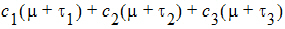
Note that c1=1, c2=0, and c3=0 generates m+t1, so m+t1 is estimable. A rearrangement of the expression is:
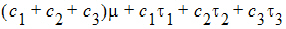
This form of the expression makes some things more obvious. For example, lj=cj for j=1,2,3. Also, any linear combination involving only ts is estimable if, and only if, l1+l2+l3=0. A linear combination of effects, where the sum of the coefficients is zero, is called a contrast. The linear combination t1 – t3 is a contrast of the t’s and thus is estimable. The linear combination t2 is not a contrast of the t’s and thus is not estimable.
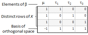
Determining estimability numerically
The X matrix for the model has three distinct rows, and these are shown in the table below. Also shown in the same table is a vector (call it z) that is a basis of the space orthogonal to the rows of X. Let l be a vector whose elements are the lj of the linear combination expression. The linear combination in vector notation is lTb and is estimable if lTZ=0. Allow for some rounding error in the computation of z. The linear combination is estimable if:
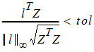
where || l ||¥ is the largest absolute value of the vector, and tol is the Estimability Tolerance.
In general, the number of rows in the basis of the space orthogonal to the rows of X is equal the number of linear dependencies among the columns of X. If there is more than one z, then previous equation must be satisfied for each z. The following table shows the basis of the space orthogonal to the rows of X.
Substitution of estimable functions for non-estimable functions
It is not always easy for a user to determine if a linear combination is estimable or not. LinMix tries to be helpful, and if a user attempts to estimate a non-estimable function, LinMix will substitute a “nearby” function that is estimable. Notice is given in the text output when the substitution is made, and it is the user's responsibility to check the coefficients to see if they are reasonable. This section is to describe how the substitution is made.
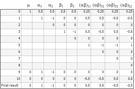
The most common attempt to estimate a non-estimable function of the parameters is probably trying to estimate a contrast of main effects in a model with interaction, so this will be used as an example. Consider the model:
where m is the over-all mean; ai is the effect of the i-th level of a factor A,i=1, 2; j is the effect of the j-th level of a factor B, j=1, 2; (ab)ij is the effect of the interaction of the i-th level of A with the j-th level of B; and the eijk are independently distributed N(0, s2). The canonical form of the QR factorization of X is displayed in rows zero through eight of the table below. The coefficients to generate a1 – a2 are shown in row 9. The process is a sequence of regressions followed by residual computations. In the m column, row 9 is already zero so no operation is done. Within the a columns, regress row 9 on row 3. (Row 4 is all zeros and is ignored.) The regression coefficient is one. Now calculate residuals: (row 9) – 1´ (row 3). This operation goes across the entire matrix, i.e., not just the a columns. The result is shown in row 10, and the next operation applies to row 10. The numbers in the b columns of row 10 are zero, so skip to the ab columns. Within the ab columns, regress row 10 on row 5. (Rows 6 through 8 are all zeros and are ignored.). The regression coefficient is zero, so there is no need to compute residuals. At this point, row 10 is a deviation of row 9 from an estimable function. Subtract the deviation (row 10) from the original (row 9) to get the estimable function displayed in the last row. The result is the expected value of the difference between the marginal A means. This is likely what the user had in mind.
This section provides a general description of the process just demonstrated on a specific model and linear combination of elements of b. Partition the QR factorization of X vertically and horizontally corresponding to the terms in X. Put the coefficients of a linear combination in a work row. For each vertical partition, from left to right, do the following:
•Regress (i.e., do a least squares fit) the work row on the rows in the diagonal block of the QR factorization.
•Calculate the residuals from this fit across the entire matrix. Overwrite the work row with these residuals.
•Subtract the final values in the work row from the original coefficients to obtain coefficients of an estimable linear combination.
QR factorization of Z scaled to canonical form
The specification of the fixed effects (as defined in “General linear mixed effects model” introduction) can contain both classification variables and continuous regressors. In addition, the model can include interaction and nested terms.
Output parameterization
Crossover example continued
Suppose X is n´p, where n is the number of observations and p is the number of columns. If X has rank p, denoted rank(X), then each parameter can be uniquely estimated. If rank(X) < p, then there are infinitely many solutions. To solve this issue, one must impose additional constraints on the estimator of b.
Suppose column j is in the span of columns 0, 1,…, j – 1. Then column j provides no additional information about the response y beyond that of the columns that come before. In this case, it seems sensible to not use the column in the model fitting. When this happens, its parameter estimate is set to zero.
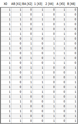
As an example, consider a simple one-way ANOVA model, with three levels. The design matrix is:
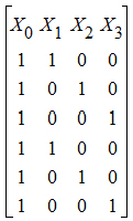
X0 is the intercept column. X1, X2, and X3 correspond to the three levels of the treatment effect. X0 and X1 are clearly linearly independent, as is X2 linearly independent of X0 and X1. But X3 is not linearly independent of X0, X1, and X2, since X3=X0 – X1 – X2. Hence b3 would be set to zero. The degrees of freedom for an effect is the number of columns remaining after this process. In this example, treatment effect has two degrees of freedom, the number typically assigned in ANOVA.
See “Residuals worksheet and predicted values” for computation details.
If intercept is in the model, then center the data. Perform a Gram-Schmidt orthogonalization process. If the norm of the vector after GS divided by the norm of the original vector is less than d, then the vector is called singular.
Transformation of the response
The Dependent Variables Transformation menu provides three options: No transformation, ln transformation (loge), or log transformation (log10). Transformations are applied to the response before model fitting. Note that all estimates using log will be the same estimates found using ln, only scaled by ln 10, since log(x)=ln(x)/ln(10).
If the standard deviation is proportional to the mean, taking the logarithm often stabilizes the variance, resulting in better fit. This implicitly assumes that the error structure is multiplicative with lognormal distribution.
The fixed effects are given in the linear combination expression. Using that model, the design matrix X would be expanded into that presented in the following table. The vector of fixed effects corresponding to that design matrix would be: b = (b0,b1,b2,b3,b4,b5,b6).
Notice that X2=X0 – X1. Hence set b2=0. Similarly, X4=X0 – X3 and X6=X0 – X5, and hence set b4=0 and b6=0.
The table below shows the design matrix expanded for a the fixed effects model Sequence + Period +Treatment.
The LinMix Variance Structure tab specifies the Z, G, and R matrices defined in “General linear mixed effects model” introduction. The user may have zero, one, or more random effects specified. Only one repeated effect may be specified. The Repeated effect specifies the R=Var(e). The Random effects specify Z and the corresponding elements of G=Var(g).
Repeated effect
Random effects
Multiple random effects vs. multiple effects on one random effect
Covariance structure types in the Linear Mixed Effects object
The repeated effect is used to model a correlation structure on the residuals. Specifying the repeated effect is optional. If no repeated effect is specified, then R=s2 IN is used, where N denotes the number of observations, and IN is the N ´ N identity matrix.
All variables used on this tab of the Linear Mixed Effects object must be classification variables.
To specify a particular repeated effect, one must have a classification model term that uniquely identifies each individual observation. Put the model term in the Repeated Specification field. Note that a model term can be a variable name, an interaction term (e.g., Time*Subject), or a nested term (e.g., Time(Subject)).
The variance blocking model term creates a block diagonal R matrix. Suppose the variance blocking model term has b levels, and further suppose that the data are sorted according to the variance blocking variable. Then R would have the form:

where S is the variance structure specified.
The variance S is specified using the Type pull-down menu. Several variance structures are possible, including unstructured, autoregressive, heterogeneous compound symmetry, and no-diagonal factor analytic. See the Help file for the details of the variance structures. The autoregressive is a first-order autoregressive model.
To model heterogeneity of variances, use the group variable. Group will accept any model term. The effect is to create additional parameters of the same variance structure. If a group variable has levels g=1, 2,…, ng, then the variance for observations within group g will be Sg.
An example will make this easier to understand. Suppose five subjects are randomly assigned to each of three treatment groups; call the treatment groups T1, T2, and T3. Suppose further that each subject is measured in periods t=0, 1, 2, 3, and that serial correlations among the measurements are likely. Suppose further that this correlation is affected by the treatment itself, so the correlation structure will differ among T1, T2, and T3. Without loss of generality, one may assume that the data are sorted by treatment group, then subject within treatment group.
First consider the effect of the group. It produces a variance structure that looks like:
where each element of R is a 15´15 block. Each Rg has the same form. Because the variance blocking variable is specified, the form of each Rg is:

I5 is used because there are five subjects within each treatment group. Within each subject, the variance structured specified is:
This structure is the autoregressive variance type. Other variance types are also possible. Often compound symmetry will effectively mimic autoregressive in cases where autoregressive models fail to converge.
The output will consist of six parameters: s2 and r for each of the three treatment groups.
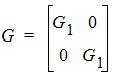
Unlike the (single) repeated effect, it is possible to specify up to 10 random effects. Additional random effects can be added by clicking Add Random. To delete a previously specified random effect, click Delete Random. It is not possible to delete all random effects; however, if no entries are made in the random effect, then it will be ignored.
Model terms entered into the Random Effects model produce columns in the Z matrix, constructed in the same way that columns are produced in the X matrix. It is possible to put more than one model term in the Random Effects Model, but each random page will correspond to a single variance type. The variance matrix appropriate for that type is sized according to the number of columns produced in that random effect.
The Random Intercept checkbox puts an intercept column (that is, all ones) into the Z matrix.
The Variance Blocking Variables has the effect of inducing independence among the levels of the Variance Blocking Variables. Mathematically, it expands the Z matrix by taking the Kronecker product of the Variance Blocking Variables with the columns produced by the intercept checkbox and the Random Effects Model terms.
The Group model term is used to model heterogeneity of the variances among the levels of the Group model term, similarly to Repeated Effects.
Multiple random effects vs. multiple effects on one random effect
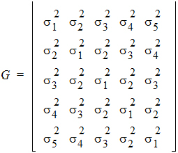
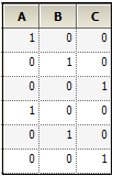
Suppose one has two random effect variables, R1 and R2. Suppose further that R1 has three levels, A, B, and C, while R2 has two levels, Y and Z. The hypothetical data are shown as follows.
•R1 values: A, B, C, A, B, C
•R2 values: Y, Y, Y, Z, Z, Z
Specifying a random effect of R1+R2 will produce different results than specifying R1 on Random 1 and R2 on Random 2 pages. This example models the variance using the compound symmetry variance type. To illustrate this, build the resulting Z and G matrices.
For R1+R2 on Random 1 page, put the columns of each variable in the Z matrix to get the following.
The random effects can be placed in a vector: g = (g1,g2,g3,g4,g5)
R1 and R2 share the same variance matrix G where:
Now, consider the case where R1 is placed on Random 1 tab, and R2 is placed on Random 2 tab. For R1, the Z matrix columns are:
For R2, the columns in the Z matrix and the corresponding G is:
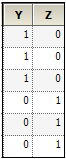
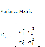
In this case:
Covariance structure types in the Linear Mixed Effects object
The Type menu in the Variance Structure tab allows users to select a variety of covariance structures. The variances of the random-effects parameters become the covariance parameters for this model. Mixed linear models contain both fixed effects and random effects parameters. For more on variance structures see “Variance structure” for an explanation of variance in linear mixed effects models. See “Covariance structure types” in the Bioequivalence section for descriptions of covariance structures.
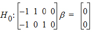
A contrast is a linear combination of the parameters associated with a term where the coefficients sum to zero. Contrasts facilitate the testing of linear combinations of parameters. For example, consider a completely randomized design with four treatment groups: Placebo, Low Dose, Medium Dose, and High Dose. The user may wish to test the hypothesis that the average of the dosed groups is the same as the average of the placebo group. One could write this hypothesis as:
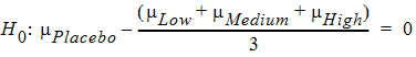
or, equivalently:

Both of these are contrasts since the sum of the coefficients is zero. Note that both contrasts make the same statement. This is true generally: contrasts are invariant under changes in scaling.
Contrasts are tested using the Wald (1943) test statistic:
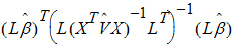
where:
• is the estimator of b.
• is the estimator of V.
•L must be a matrix such that each row is in the row space of X.
This requirement is enforced in the wizard. The Wald statistic is compared to an F distribution with rank(L) numerator degrees of freedom and denominator degrees of freedom estimated by the program or supplied by the user.
Joint versus single contrasts
Nonestimability of contrasts
Degrees of freedom
Other options
Joint contrasts are constructed when the number of columns for contrast is changed from the default value of one to a number larger than one. Note that this number must be no more than one less than the number of distinct levels for the model term of interest. This tests both hypotheses jointly, i.e., in a single test with a predetermined level of the test.
A second approach would be to put the same term in the neighboring contrast, both of which have one column. This approach will produce two independent tests, each of which is at the specified level.
To see the difference, compare Placebo to Low Dose and Placebo to Medium Dose. Using the first approach, enter the coefficients as follows.
Title = Join tests
Effect = Treatment
Contrast = Treatment
#1 Placebo –1 –1
#2 Low Dose 1 0
#3 Medium Dose 0 1
#4 High Dose 0 0
This will produce one test, testing the following hypothesis.
Now compare this with putting the second contrast in its own contrast.
Contrast #1
Title Low vs. Placebo
Effect Treatment
Contrast Treatment
#1 Placebo –1
#2 Low Dose 1
#3 Medium Dose 0
#4 High Dose 0
Contrast #2
Title Medium vs. Placebo
Effect Treatment
Contrast Treatment
#1 Placebo –1
#2 Low Dose 0
#3 Medium Dose 1
#4 High Dose 0
This produces two tests:

Note that this method inflates the overall Type I error rate to approximately 2a, whereas the joint test maintains the overall Type I error rate to a, at the possible expense of some power.
If a contrast is not estimable, then an estimable function will be substituted for the nonestimable function. See “Substitution of estimable functions for non-estimable functions” for the details.
The User specified degrees of freedom checkbox available on the Contrasts, Estimates, and Least Squares Means tabs, allows the user to control the denominator degrees of freedom in the F approximation. The numerator degrees of freedom is always calculated as rank(L). If the checkbox is not selected, then the default denominator degrees of freedom will be used. The default calculation method of the degrees of freedom is controlled on the General Options tab and is initially set to Satterthwaite.
Note:For a purely fixed effects model, Satterthwaite and residual degrees of freedom yield the same number. For details of the Satterthwaite approximation, see “Satterthwaite approximation for degrees of freedom”.
To override the default degrees of freedom, select the checkbox and type an appropriate number in the field. The degrees of freedom must greater than zero.
To control the estimability tolerance, enter an appropriate tolerance in the Estimability Tolerance field. For more information see “Substitution of estimable functions for non-estimable functions”.
The Show Coefficients checkbox produces extra output, including the coefficients used to construct the tolerance. If the contrast entered is estimable, then it will repeat the contrasts entered. If the contrasts are not estimable, it will enter the estimable function used instead of the nonestimable function.
The Estimates tab produces estimates output instead of contrasts. As such, the coefficients need not sum to zero. Additionally, multiple model terms may be included in a single estimate.
Unlike contrasts, estimates do not support joint estimates. The intervals are marginal. The level must be between zero and 100. Note that it is entered as a percent: Entering 0.95 will yield a very narrow interval with coverage just less than 1%.
All other options act similarly to the corresponding options in the Contrasts tab.
Sometimes a user wants to see the mean response for each level of a classification variable or for each combination of levels for two or more classification variables. If there are covariables with unequal means for the different levels, or if there are unbalanced data, the subsample means are not estimates that can be validly compared. This section describes least squares means, statistics that make proper adjustments for unequal covariable means and unbalanced data in the linear mixed effects model.
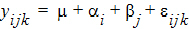
Consider a completely randomized design with a covariable. The model is:
where yij is the observed response on the jth individual on the ith treatment; ai is the intercept for the ith treatment; xij is the value of the covariable for the jth individual in the ith treatment; b is the slope with respect to x; and eij is a random error with zero expected value. Suppose there are two treatments; the average of the x1j is 5; and the average of the x2j is 15. The respective expected values of the sample means are a1+5b and a2+15b. These are not comparable because of the different coefficients of b. Instead, one can estimate a1+10b and a2+10b where the overall mean of the covariable is used in each linear combination.
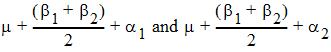
Now consider a 2 ´ 2 factorial design. The model is:
where yijk is the observed response on the kth individual on the ith level of factor A and the jth level of factor B; m is the over-all mean; ai is the effect of the ith level of factor A; bj is the effect of the jth level of factor B; and eijk is a random error with zero expected value. Suppose there are six observations for the combinations where i=j and four observations for the combinations where i ¹ j. The respective expected values of the averages of all values on level 1 of A and the averages of all values on level 2 of A are m + (0.6 b1 + 0.4 b2) + a1 and m + (0.4 b1 + 0.6 b2) + a2. Thus, sample means cannot be used to compare levels of A because they contain different functions of b1 and b2. Instead, one compares the linear combinations:
The preceding examples constructed linear combinations of parameters, in the presence of unbalanced data, that represent the expected values of sample means in balanced data. This is the idea behind least squares means. Least squares means are given in the context of a defining term, though the process can be repeated for different defining terms for the same model. The defining term must contain only classification variables and it must be one of the terms in the model. Treatment is the defining term in the first example, and factor A is the defining term in the second example. When the user requests least squares means, LinMix automatically generates the coefficients lj of the linear combination expression and processes them almost as it would process the coefficients specified in an estimate statement. This chapter describes generation of linear combinations of elements of b that represent least squares means. A set of coefficients are created for each of all combinations of levels of the classification variables in the defining term. For all variables in the model, but not in the defining term, average values of the variables are the coefficients. The average value of a numeric variable (covariable) is the average for all cases used in the model fitting. For a classification variable with k levels, assume the average of each indicator variable is 1/k. The value 1/k would be the actual average if the data were balanced. The values of all variables in the model have now been defined. If some terms in the model are products, the products are formed using the same rules used for constructing rows of the X matrix as described in the “Fixed effects” section. It is possible that some least squares means are not estimable.
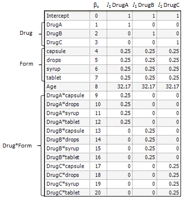
For example, suppose the fixed portion of the model is: Drug + Form + Age + Drug*Form
To get means for each level of Drug, the defining term is Drug. Since Drug has three levels, three sets of coefficients are created. Build the coefficients associated the first level of Drug, DrugA. The first coefficient is one for the implied intercept. The next three coefficients are 1, 0, and 0, the indicator variables associated with DrugA. Form is not in the defining term, so average values are used. The next four coefficients are all 0.25, the average of a four factor indicator variable with balanced data. The next coefficient is 32.17, the average of Age. The next twelve elements are:
The final result is shown in the DrugA column in the following table. The results for DrugB and DrugC are also shown in the table. No new principles would be illustrated by finding the coefficients for the Form least squares means. The coefficients for the Drug*Form least squares means would be like representative rows of X except that Age would be replaced by the average of Age.
Comparing the Linear Mixed Effects object to SAS PROC MIXED
The following outlines differences between LinMix and PROC MIXED in SAS.
Degrees of freedom
LinMix: Uses Satterthwaite approximation for all degrees of freedom, by default. User can also select Residual.
PROC MIXED: Chooses different defaults based on the model, random, and repeated statements. To match LinMix, set the SAS ‘ddfm=satterth’ option.
Multiple factors on the same random command
LinMix: Effects associated with the matrix columns from a single random statement are assumed to be correlated per the variance specified. Regardless of variance structure, if random effects are correlated, put them on the same random tab; if independent, put them on separate tabs.
PROC MIXED: Similar to LinMix, except it does not follow this rule in the case of Variance Components, so LinMix and SAS will differ for models with multiple terms on a random statement using the VC structure.
REML
LinMix: Uses REML (Restricted Maximum Likelihood) estimation, as defined in Corbeil and Searle (1976), does maximum likelihood estimation on the residual vector.
PROC MIXED: Modifies the REML by ‘profiling out’ residual variance. To match LinMix, set the ‘noprofile’ option on the PROC MIXED statement. In particular, LinMix –log(likelihood) may not equal twice SAS ‘–2 Res Log Like’ if noprofile is not set.
Akaike and Schwarz’s criteria
LinMix: Uses the smaller-is-better form of AIC and SBC in order to match Phoenix.
PROC MIXED: Uses the bigger-is-better form. In addition, AIC and SBC are functions of the likelihood, and the likelihood calculation method in LinMix also differs from SAS.
Saturated variance structure
LinMix: If the random statement saturates the variance, the residual is not estimable. Sets the residual variance to zero. A user-specified variance structure takes priority over that supplied by LinMix.
PROC MIXED: Sets the residual to some other number. To match LinMix, add the SAS residual to the other SAS variance parameter estimates.
Convergence criteria
LinMix: The convergence criterion is gT H–1g < tolerance with H positive definite, where g is the gradient and H is the Hessian of the negative log-likelihood.
PROC MIXED: The default convergence criterion options are ‘convh’ and ‘relative’. The LinMix criterion is equivalent to SAS with the ‘convh’ and ‘absolute’ options set.
Modified likelihood
LinMix: Tries to keep the final Hessian (and hence the variance matrix) positive definite. Determines when the variance is over-specified and sets some parameters to zero.
PROC MIXED: Allows the final Hessian to be nonpositive definite, and hence will produce different final parameter estimates. This often occurs when the variance is over-specified (i.e., too many parameters in the model).
Keeping VC positive
LinMix: For VC structure, LinMix keeps the final variance matrix positive definite, but will not force individual variances > 0.
PROC MIXED: If a negative variance component is estimated, 0 is reported in the output.
Partial tests of model effects
LinMix: The partial tests in LinMix are not equivalent to the Type III method in SAS though they coincide in most situations. See “Partial Tests worksheet”.
PROC MIXED: The Type III results can change depending on how one specifies the model. For details, consult the SAS manual.
Not estimable parameters
LinMix: If a variable is not estimable, ‘Not estimable’ is reported in the output. LinMix provides the option to write out 0 instead.
PROC MIXED: SAS writes the value of 0.
ARH, CSH variance structures
LinMix: Uses the standard deviations for the parameters, and prints the standard deviations in the output.
PROC MIXED: Prints the variances in the output for final parameters, though the model is expressed in terms of standard deviations.
CS variance structure
LinMix: Does not estimate a Residual parameter, but includes it in the csDiag parameter.
PROC MIXED: Estimates Residual separately. csDiag = Variance + Residual in SAS.
UN variance structure
LinMix: Does not estimate a Residual parameter, but includes it in the diagonal term of the UN matrix.
PROC MIXED: Estimates Residual separately. UN (1,1) = UN(1,1) + Residual in SAS, etc. (If a weighting variable is used, the Residual is multiplied by 1/weight.)
Repeated without any time variable
LinMix: Requires an explicit repeated model. To run some SAS examples, a time variable needs to be added.
PROC MIXED: Does not require an explicit repeated model. It instead creates an implicit time field and assumes data are sorted appropriately.
Group as classification variable
LinMix: Requires variables used for the subject and group options to be declared as classification variables.
PROC MIXED: Allows regressors, but requires data to be sorted and considers each new regressor value to indicate a new subject or group. Classification variables are treated similarly.
Singularity tolerance
LinMix: Define dii as the i-th diagonal element of the QR factorization of X, and Dii the sum of squares of the i-th column of the QR factorization. The i-th column of X is deemed linearly dependent on the proceeding columns if dii2 < (singularity tolerance)´Dii. If intercept is present, the first row of Dii is omitted.
PROC MIXED: Define dii as the diagonal element of the XTX matrix during the sweeping process.
If the absolute diagonal element |dii| < (singularity tolerance)´Dii, where Dii is the original diagonal of XTX, then the parameter associated with the column is set to zero, and the parameter estimates are flagged as biased.
Allen and Cady (1982). Analyzing Experimental Data By Regression. Lifetime Learning Publications, Belmont, CA
Corbeil and Searle (1976). Restricted maximum likelihood (REML) estimation of variance components in the mixed models, Technometrics, 18:31–8
Fletcher (1980). Practical methods of optimization, Vol. 1: Unconstrained Optimization. John Wiley & Sons, New York
Giesbrecht and Burns (1985). Two-stage analysis based on a mixed model: Large sample asymptotic theory and small-sample simulation results. Biometrics 41:477–86
Gill, Murray and Wright (1981). Practical Optimization. Academic Press
Wald (1943). Tests of statistical hypotheses concerning several parameters when the number of observations is large. Transaction of the American Mathematical Society 54
