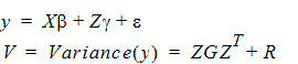
Linear mixed effects computations
The following sections cover the methods the Linear Mixed Effects object uses to create model results.
Restricted maximum likelihood
Newton algorithm for maximization of restricted likelihood
Starting values
Convergence criterion
Satterthwaite approximation for degrees of freedom
Linear mixed effects scenario
For linear mixed effects models that contain random effects, the first step in model analysis is determining the maximum likelihood estimates of the variance parameters associated with the random effects. This is accomplished in LinMix using Restricted Maximum Likelihood (REML) estimation.
The linear mixed effects model described under “General linear mixed effects model” is:
Let q be a vector consisting of the variance parameters in G and R. The full maximum likelihood procedure (ML) would simultaneously estimate both the fixed effects parameters b and the variance parameters q by maximizing the likelihood of the observations y with respect to these parameters. In contrast, restricted maximum likelihood estimation (REML) maximizes a likelihood that is only a function of the variance parameters q and the observations y, and not a function of the fixed effects parameters. Hence for models that do not contain any fixed effects, REML would be the same as ML.
To obtain the restricted likelihood function in a form that is computationally efficient to solve, the data matrix [X | Z | y] is reduced by a QR factorization to an upper triangular matrix. Let [R0 | R1 | R2] be an orthogonal matrix such that the multiplication with [X | Z | y] results in an upper triangular matrix:
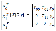
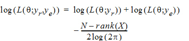
REML estimation maximizes the likelihood of q based on yr and ye of the reduced data matrix, and ignores y0. Since ye has a distribution that depends only on the residual variance, and since yr and ye are independent, the negative of the log of the restricted likelihood function is the sum of the separate negative log-likelihood functions:
where:
log(L(q; yr))=–½ log (|Vr |) – ½ yr T Vr –1 yr
log(L(q; ye))=–ne/2 log(qe) – ½ (yeTye/qe)
Vr is the Variance(yr)
qe is the residual variance
ne is the residual degrees of freedom
N is the number of observations used
For some balanced problems, ye is treated as a multivariate residual: [ye1 | ye2 | ... | yen]
in order to increase the speed of the program and then the log-likelihood can be computed by the equivalent form:
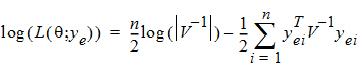
where V is the dispersion matrix for the multivariate normal distribution.
For more information on REML, see Corbeil and Searle (1976).
Newton algorithm for maximization of restricted likelihood
Newton’s algorithm is an iterative algorithm used for finding the minimum of an objective function. The algorithm needs a starting point, and then at each iteration, it finds the next point using:
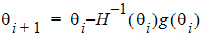
where H–1 is the inverse of the Hessian of the objective function, and g is the gradient of the objective function.
The algorithm stops when a convergence criterion is met, or when it is unable to continue.
In the Linear Mixed Effects object, a modification of Newton’s algorithm is used to minimize the negative restricted log-likelihood function with respect to the variance parameters q, hence yielding the variance parameters that maximize the restricted likelihood. Since a constant term does not affect the minimization, the objective function used in the algorithm is the negative of the restricted log-likelihood without the constant term.

Newton’s algorithm is modified by adding a diagonal matrix to the Hessian when determining the direction vector for Newton’s, so that the diagonal matrix plus the Hessian is positive definite, ensuring a direction of descent.
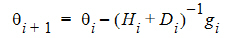
The appropriate Di matrix is found by a modified Cholesky factorization as described in Gill, Murray and Wright (1981). Another modification to Newton’s algorithm is that, once the direction vector, d = –(Hi + Di)–1gi, has been determined, a line search is done as described in Fletcher (1980) to find an approximate minimum along the direction vector.
Note from the discussion on REML estimation that the restricted log-likelihood is a function of the variance matrix Vr and the residual variance, which are in turn functions of the parameters q. The gradient and Hessian of the objective function with respect to q are therefore functions of first and second derivatives of the variances with respect to q. Since the variances can be determined through the types specified for G and R (e.g., Variance Components, Unstructured, etc.), the first and second derivatives of the variance can be evaluated in closed-form, and hence the gradient and Hessian are evaluated in closed-form in the optimization algorithm.
Newton’s algorithm requires initial values for the variance parameter q. The user can supply these in the Linear Mixed Effects object’s General Options tab, by clicking the Generate button under Initial Variance Parameters. More often, LinMix will determine initial values. For variance structures that are linear in q (Variance Components, Unstructured, Compound Symmetry, and Toeplitz), the initial values are determined by the method of moments. If the variance structure is nonlinear, then LinMix will calculate a “sample” variance by solving for random effects and taking their sums of squares and cross-products. The sample variance will then be equated with the parametric variance, and the system of equations will be solved to obtain initial parameter estimates. If either method fails, LinMix will use values that should yield a reasonable variance matrix, e.g., 1.0 for variance components and standard deviations, 0.01 for correlations.
Sometimes the method of moments will yield estimates of q that are REML estimates. In this case the program will not need to iterate.
The convergence criterion used in the Linear Mixed Effects object is that the algorithm has converged if: gT(q)H-1(q)g(q) < i, where i is the convergence criterion specified on the General Options tab. The default is 1´10–10.
The possible convergence outcomes from Newton’s algorithm are:
•Newton's algorithm converged with a final Hessian that is positive definite, indicating successful convergence at a local, and hopefully global, minimum.
•Newton's algorithm converged with a modified Hessian, indicating that the model may be over-specified. The output is suspect. The algorithm converged, but not at a local minimum. It may be in a trough, at a saddle point, or on a flat surface.
•Initial variance matrix is not positive definite. This indicates an invalid starting point for the algorithm.
•Intermediate variance matrix is not positive definite. The algorithm cannot continue.
•Failed to converge in allocated number of iterations.
Satterthwaite approximation for degrees of freedom
The linear model used in linear mixed effects modeling is: Y ~ N(Xb,V)
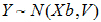
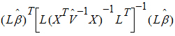
where X is a matrix of fixed known constants, b is an unknown vector of constants, and V is the variance matrix dependent on other unknown parameters. Wald (1943) developed a method for testing hypotheses in a rather general class of models. To test the hypothesis H0: Lb=0, the Wald statistic is:
where:
 is the estimator of b.
 is the estimator of V.
L must be a matrix such that each row is in the row space of X.
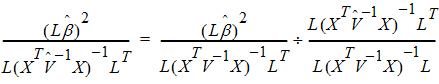
The Wald statistic is asymptotically distributed under the null hypothesis as a chi-squared random variable with q=rank(L) degrees of freedom. In common variance component models with balanced data, the Wald statistic has an exact F-distribution. Using the chi-squared approximation results in a test procedure that is too liberal. LinMix uses a method based on analysis techniques described by Allen and Cady (1982) for finding an F distribution to approximate the distribution of the Wald statistic.
Giesbrecht and Burns (1985) suggested a procedure to determine denominator degrees of freedom when there is one numerator degree of freedom. Their methodology applies to variance component models with unbalanced data. Allen derived an extension of their technique to the general mixed model.
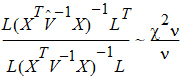
A one degree of freedom (df) test is synonymous with L having one row in the previous equation. When L has a single row, the Wald statistic can be re-expressed as:
Consider the right side of this equation. The distribution of the numerator is approximated by a chi-squared random variable with 1 df. The objective is to find n such that the denominator is approximately distributed as a chi-squared variable with n df. If:
is true, then:
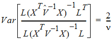
The approach is to use this equation to solve for n.
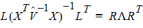
Find an orthogonal matrix R and a diagonal matrix L such that:
The Wald statistic equation can be re-expressed as:
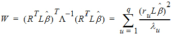
where ru is the u-th column of R, and lu is the u-th diagonal of L.
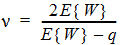
Each term in the previous equation is similar in form to the Wald statistic equation for a single row. Assuming that the u-th term is distributed F(1, nu), the expected value of W is:
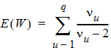
Assuming W is distributed F(q, n), its expected value is qn/(n – 2). Equating expected values and solving for n, one obtains:
The following example is used as a framework for discussing the functions and computations of the Linear Mixed Effects object.
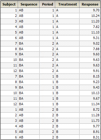
An investigator wants to estimate the difference between two treatments for blood pressure, labeled A and B. Because responses are fairly heterogeneous among people, the investigator decided that each study subject will be his own control, which should increase the power of the study. Therefore, each subject will be exposed to treatments A and B. Since the treatment order might affect the outcome, half the subjects will receive A first, and the other half will receive B first. For the analysis, note that this crossover study has two periods, 1 and 2, and two sequence groups AB and BA.
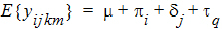
The model will be of the form:

where:
i is the period index (1 or 2)
j is the sequence index (AB or BA)
k is the subject within sequence group index (1…nj)
m is the observation within subject index (1, 2)
q is the treatment index (1, 2)
m is the intercept
pi is the effect due to period
dj is the effect due to sequence grouping
tq is the effect due to treatment, the purpose of the study
Sk(j) is the effect due to subject
eijkm is the random variation
Typically, eijkm is assumed to be normally distributed with mean zero and variance s2 > 0. The purpose of the study is to estimate t1 – t2 in all people with similar inclusion criteria as the study subjects. Study subjects are assumed to be randomly selected from the population at large. Therefore, it is desirable to treat subject as a random effect. Hence, assume that subject effect is normally distributed with mean zero and variance Var(Sk(j)) ³ 0.
This mixing of the regression model and the random effects is known as a mixed effect model. The mixed effect model allows one to model the mean of the response as well as its variance. Note that in the model equation above, the mean is:
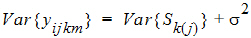
and the variance is given by:
E{yijkm} is known as the fixed effects of the model, while Sk(j)+eijkm constitutes the random effects, since these terms represent random variables whose variances are to be estimated. A model with only the residual variance is known as a fixed effect model. A model without the fixed effects is known as a random effect model. A model with both is a mixed effect model.
The data are shown in the table below. The Linear Mixed Effects object is used to analyze these data. The fixed and random effects of the model are entered on different tabs of the Diagram view. This is appropriate since the fixed effects model the mean of the response, while the random effects model the variance of the response.
The Linear Mixed Effects object can fit linear models to Gaussian data. The mean and variance structures can be simple or complex. Independent variables can be continuous or discrete, and no distributional assumption is made about them.
This model provides a context for the linear mixed effects model.
