Bioequivalence is said to exist when a test formulation has a bioavailability that is similar to that of the reference. There are three types of bioequivalence: Average, Individual, and Population. Average bioequivalence states that average bioavailability for test formulation is the same as for the reference formulation. Population bioequivalence is meant to assess equivalence in prescribability and takes into account both differences in mean bioavailability and in variability of bioavailability. Individual bioequivalence is meant to assess switchability of products, and is similar to population bioequivalence.
The US FDA Guidance for Industry (January 2001) recommends that a standard in vivo bioequivalence study design be based on the administration of either single or multiple doses of the test and reference products to healthy subjects on separate occasions, with random assignment to the two possible sequences of drug product administration. Further, the 2001 guidance recommends that statistical analysis for pharmacokinetic parameters, such as area under the curve (AUC) and peak concentration (Cmax) be based on a test procedure termed the two one-sided tests procedure to determine whether the average values for pharmacokinetic parameters were comparable for test and reference formulations. This approach is termed average bioequivalence and involves the calculation of a 90% confidence interval for the ratio of the averages of the test and reference products. To establish bioequivalence, the calculated interval should fall within a bioequivalence limit, usually 80–125% for the ratio of the product averages. In addition to specifying this general approach, the 2001 guidance also provides specific recommendations for (1) logarithmic transformations of pharmacokinetic data, (2) methods to evaluate sequence effects, and (3) methods to evaluate outlier data.
It is also recommended that average bioequivalence be supplemented by population and individual bioequivalence. Population and individual bioequivalence include comparisons of both the averages and variances of the study measure. Population bioequivalence assesses the total variability of the measure in the population. Individual bioequivalence assesses within-subject variability for the test and reference products as well as the subject-by-formulation interaction.
Bioequivalence between two formulations of a drug product, sometimes referred to as relative bioavailability, indicates that the two formulations are therapeutically equivalent and will provide the same therapeutic effect. The objectives of a bioequivalence study is to determine whether bioequivalence exists between a test formulation and reference formulation and to identify whether the two formulations are pharmaceutical alternatives that can be used interchangeably to achieve the same effect.
Bioequivalence studies are important because establishing bioequivalence with an already approved drug product is a cost-efficient way of obtaining drug approval. Bioequivalence studies are also useful for testing new formulations of a drug product, new routes of administration of a drug product, and for a drug product that has changed after approval.
There are three different types of bioequivalence: average bioequivalence, population bioequivalence, and individual bioequivalence. All types of bioequivalence comparisons are based on the calculation of a criterion (or point estimate), on the calculation of an interval for the criterion, and on a predetermined acceptability limit for the interval.
A procedure for establishing average bioequivalence involves administration of either single or multiple doses of the test and reference formulations to subjects, with random assignment to the possible sequences of drug administration. Then a statistical analysis of pharmacokinetic parameters such as AUC and Cmax is done on a log-transformed scale to determine the difference in the average values of these parameters between the test and reference data, and to determine the interval for the difference. To establish bioequivalence, the interval, usually calculated at the 90% level, should fall within a predetermined acceptability limit, usually within 20% of the reference average. An equivalent approach using two, one-sided t-tests is also recommended. Both the interval approach and the two one-sided t-tests are described further below.
The average bioequivalence should be supplemented by population and individual bioequivalences. These added approaches are needed because average bioequivalence uses only a comparison of averages, and not the variances, of the bioequivalence measures. In contrast, population and individual bioequivalence approaches include comparisons of both the averages and variances of the study measure. The population bioequivalence approach assesses the total variability of the study measure in the population. The individual bioequivalence approach assesses within-subject variability for the test and reference products as well as the subject-by-formulation interaction.
The concepts of population and individual bioequivalence are related to two types of drug interchangeability: prescribability and switchability. Drug prescribability refers to when a physician prescribes a drug product to a patient for the first time, and must choose from a number of bioequivalent drug products. Drug prescribability is usually assessed by population bioequivalence. Drug switchability refers to when a physician switches a patient from one drug product to a bioequivalent product, such as when switching from an innovator drug product to a generic substitute within the same patient. Drug switchability is usually assessed by individual bioequivalence.
The covariance types used in the Bioequivalence model object are the same as those used in the Linear Mixed Effects model object. For more on variance structures see “Variance structure” in the LinMix section. Covariance types must be specified if the model contains random effects.
The Variance Structure tab in the Bioequivalence object allows users to select the covariance type used in the model. The variances of the random-effects parameters become the covariance parameters for a bioequivalence model that contains both fixed effect and random effect parameters.
The choices for covariance structures are listed below. The list uses the following notation:
n: number of groups. n=1 if the group option is not used.
t: number of time points in the repeated context.
b: dimension parameter: for some variance structures, the number of bands; for others, the number of factors.
1(expression): 1 if the expression is true, 0 if the expression is false.
Variance Components have n parameters; ith, jth element:
sk21(i = j)
i corresponds to kth effect
Unstructured has n x t x (t + 1)/2 parameters; ith, jth element:
sij
in output, sii = un(i,j)
Banded Unstructured (b) has n x b/2(2t – b +1) parameters, if b < t; otherwise, same as Unstructured; ith, jth element:
sij(|i – j| < n)
Compound Symmetry has n x 2 parameters; ith, jth element:
s21 + s21(i = j)
in output, s2 = csDiag, s2i = csBlock
Heterogeneous Compound Symmetry has n x (t + 1) parameters; ith, jth element:
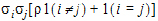
in output, si = cshSD(i), r = cshCorr
Autoregressive (1) has n x 2 parameters; ith, jth element:
s2r|i – j|
in output, s2 = arVar, r = arCorr
Heterogeneous Autoregressive (1) has n x (t + 1) parameters; ith, jth element:
sisjr|i – j|
in output, si = arhSD(i), r = arhCorr
No-Diagonal Factor Analytic has n x t(t + 1)/2 parameters; ith, jth element:
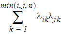
in output, lik = lambda(i,k)
Banded No-Diagonal Factor Analytic (b) has n x b/2(2t – b + 1) parameters if b < t; otherwise, same as No-Diagonal Factor Analytic; ith, jth element:
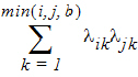
in output, lik = lambda(i,k)
The limits and constraints discussed here are for Bioequivalence and Linear Mixed Effects modeling.
Cell data may not include question marks (?) or either single (') or double (“) quotation marks.
Variable names must begin with a letter. After the first character, valid characters include numbers and underscores (my_file_2). They cannot include spaces or the following operational symbols: +, –, *, /, =. They also cannot include parentheses (), question marks (?), semicolons (;), single or double quotes.
Titles (in Contrasts, Estimates, or ASCII) can have single or double quotation marks, but not both.
The following are maximum counts for variables.
model terms 30
factors in a model term 10
sort keys 16
dependent variables 128
covariate/regressor variables 255
variables in the dataset 256
levels per variable 1,000
random and repeated statements 10
contrast statements 100
estimate statements 100
combined length of all variance parameter names (total characters) 10,000
combined length of all level names (total characters) 10,000
combined length of input data line (total characters in line of data or column headers) 2,500
