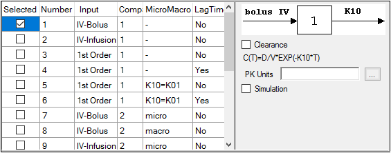
The Model Selection tab for most of the Least-Squares Regression Models allows users to select a model and whether or not the model uses simulated data/clearance parameter. (For the User ASCII Model, the Model Selection tab contains weighting options as described in the “Weighting/Dosing Options tab” description.)
-
Check the checkbox beside the model number to choose it. For Dissolution models, click an option button to select a model.
Refer to any of the following sections for model details:
Linear models
Michaelis-Menten models
Pharmacodynamic models
Pharmacokinetic models
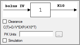
Selecting a model displays a diagram beside the model selection menu that describes the model’s functions. The model’s equation is listed beneath the diagram.
-
Set the options for the selected model.
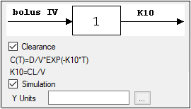
•For Indirect Response, PK, and PK/PD Linked models, select the Clearance checkbox to add a clearance parameter to the model. (The clearance parameter option is not available for PK models 8, 10, 13, 14, 17, 18, or 19.)
•For Michaelis-Menten Models, use the Number of Constants box to type or select the number of dosing constants used per profile. (For more on how the number of constants corresponds to the number, amount, and time of doses, see “Dosing constants for the Michaelis-Menten model”.)
•For PK/PD Linked Models, enter concentration units in the PK Units text field or click the Units Builder […] button to use the Units Builder dialog.
Note:For PK/PD Linked Models, to view all PK parameter units in the PK Parameters panel, users must supply concentration units in the PK Units text field in the Model Selection tab and dose units in the Weighting/Dosing Options tab.
-
Check the Simulation checkbox to simulate concentration data. Enter units for the simulated data in the Y Units text field or click the Units Builder […] button to use the Units Builder dialog.
If the Simulation checkbox is selected then no concentration variable is required to run the model.
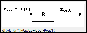
The Linked Model tab allows users to select the model to link with model specified in the Model Selection tab. It is available only for the Indirect Response and PK/PD Linked Models.

-
Check the checkbox beside the model number to choose it.
For more on these models, see “Indirect Response models”. For PK/PD Linked Models, see “Pharmacodynamic models”.
For a list of PD output parameters used in linked PK/PD models, see “PD output parameters in a PK/PD model”.
Selecting a model displays a diagram beside the model selection menu that describes the model’s functions. The model’s equation is listed beneath the diagram.
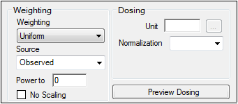
The Weighting Options tab (in Dissolution, Linear, M-M, and PD Model objects) and the Weighting/Dosing Options tab (in Indirect Response, PK, and PK/PD Linked Model objects) allows users to select a weighting scheme and specify and preview dosing options.
-
Use the Weighting menu to select one of six weighting schemes:
User Defined: Weights are read from a column in the dataset.
Uniform: Users can enter custom observed to or predicted to the power of N values. If selected, then users must select Observed or Predicted in the Source menu and type the power value in the Power to text field.
1/Y: Weight the data by 1/observed Y.
1/Yhat: Weight the data by 1/predicted Y (iterative reweighting).
1/(Y*Y): Weight the data by 1/observed Y2.
1/(Yhat*Yhat): Weight the data by 1/predicted Y2 (iterative reweighting).
-
Use the Source menu to select one of three weighting sources:
Source: Selecting this option sets the weighting to User Defined and adds a Weight column to the Main Mappings panel. If selected, users must map the weighting column in the dataset to the Weight context in the Main Mappings panel.
Observed: Select to use weighted least squares. This is the default selection for 1/Y and 1/(Y*Y). The default power for 1/Y is –1 and for 1/(Y*Y) it is –2.
Predicted: Select to use iterative reweighting. This is the default selection for 1/Yhat and 1/(Yhat*Yhat). The default power for 1/Yhat is –1 and for 1/(Yhat*Yhat) it is –2.
-
Type a power value in the Power to text field. (This option is disabled if Source is set to Source.)
Entering -1 automatically sets the weighting to 1/Y (if Observed is the source) or 1/Yhat (if Predicted is the source).
Entering -2 automatically sets the weighting to 1/(Y*Y) (if Observed is the source) or 1/(Yhat*Yhat) (if Predicted is the source).
-
Check the No Scaling checkbox to not scale the weighting for observed weighting values.
When weights are contained in a dataset or Observed is selected as the source, the weights for individual data values are scaled so that the sum of weights for each function is equal to the number of data values. Weights must not be 0 (zero) in order to scale.
Scaling has no effect on the model fitting, because the weights of the observations are proportionally the same. However, scaling weights provides increased numerical stability.
Available for Indirect Response, PK, and PK/PD Linked models.
-
Enter the dosing unit in the Unit text field or click the […] button to use the Units Builder dialog to set the dosing unit.
Note:For Indirect Response Models, to view all PK parameter units in the PK Parameters panel, users must supply units for the time and concentration data in the input and specifying dose units in the Weighting/Dosing Options tab.
For PK/PD Linked Models, to view all PK parameter units in the PK Parameters panel, users must supply concentration units in the PK Units text field in the Model Selection tab and dose units in the Weighting/Dosing Options tab.
-
Use the Normalization menu to select the appropriate factor, if the dose amount is normalized by subject body weight or body mass index. Options include: None, kg, g, mg, m**2, 1.73 m**2.
Dose normalization usage:
•If doses are in milligrams per kilogram of body weight, select mg as the dosing unit and kg as the dose normalization.
•The Normalization menu affects the output parameter units. For example, if dose volume is in liters, selecting kg as the dose normalization changes the units to L/kg.
•Dose normalization affects units for all volume and clearance parameters in PK models.
-
Type the number of doses per profile into the # Doses text field. (Only enabled if an internal worksheet is used for Dosing.)
If different profiles require different numbers of doses, enter the highest number of doses. -
Click Preview Dosing to view a preview of dose option selections.
If an external dosing data worksheet is used to provide dosing data, then the preview window will show the number of doses and dosing time points per profile. Click OK to close the preview window.
All iterative estimation procedures require initial estimates of the parameter values. Phoenix computes initial estimates via curve stripping for single-dose models. For all other situations, including multiple-dose models, users must provide initial estimates or boundaries to be used by Phoenix in creating initial estimates. Parameter boundaries provide a basis for grid searching initial parameter estimates, and also limit the estimates during modeling. This is useful if the values become unrealistic or the model does not converge. For more on setting initial parameter estimates, refer to “Parameter Estimates and Boundaries Rules”.

Set the parameter calculation method:
Note:The default minimization method, Gauss-Newton (Hartley) (located in the Engine Settings tab), and the Parameter Boundaries option Do Not Use Bounds are recommended for all Linear models.
-
Select the User Supplied Initial Parameter Values option button to enter initial parameter estimates in the Initial Estimates panel.
Or
Select the WinNonlin Generated Initial Parameter Values option button to have Phoenix determine the initial parameter values.
•If the User Supplied Bounds option button is selected, Phoenix uses curve stripping to provide initial estimates. If curve stripping fails, then Phoenix uses the grid search method.
•If the WinNonlin Bounds option button is selected, Phoenix uses curve stripping to provide initial estimates, and then applies boundaries to the model parameters for model fitting. If curve stripping fails, the model fails because Phoenix cannot use grid search for initial estimates without user-supplied boundaries.
-
Check the Propagate Final Estimates checkbox to propagate initial parameter estimates across all sort levels.
This option is available when more than one sort variable is used in the main dataset.
If this option is selected, then initial estimates and boundaries are entered or mapped only for the first sort level. The final parameter estimates from the first sort level provide the initial estimates for each consecutive sort level.
Set the boundary calculation method:
Parameter boundaries provide a basis for grid searching initial parameter estimates, and also limit the estimates during modeling. This is useful if the values become unrealistic or the model does not converge. For more on using parameter boundaries, refer to “Parameter Estimates and Boundaries Rules”.
-
Select the User Supplied Initial Bounds option to enter parameter boundaries in the Initial Estimates panel.
Or select the WinNonlin Bounds option to have Phoenix determine the parameter boundaries.
Or select the Do No Use Bounds option to not use parameter boundaries.
The Engine Settings tab provides control over the model fitting algorithm and related settings.

-
Use the Minimization menu to select the method to use with the Indirect Response model.
Method 1: The Nelder-Mead algorithm does not require the estimated variance-covariance matrix as part of its algorithm, so it often performs very well on ill-conditioned datasets. Ill-conditioned indicates that, for the given dataset and model, there is not enough information contained in the data to precisely estimate all of the parameters in the model or that the sum of squares surface is highly curved. Although the procedure works well, it can be slow, particularly when used to fit a system of differential equations.
Method 2: Gauss-Newton (Levenberg and Hartley) is the default algorithm and performs well on a wide class of problems, including ill-conditioned datasets. Although the Gauss-Newton method does require the estimated variance-covariance matrix of the parameters, the Levenberg modification suppresses the magnitude of the change in parameter values from iteration to iteration to a reasonable amount. This enables the method to perform well on ill-conditioned datasets.
Method 3: Gauss-Newton (Hartley) is another Gauss-Newton method. It is not as robust as Methods 1 and 2 but is extremely fast. Method 3 is recommended when speed is a consideration or when maximum likelihood estimation or linear regression analysis is to be performed. It is not recommended for fitting complex models.
Note:The use of bounds is recommended with Methods 2 and 3. For linear regressions, use Method 3 without bounds.
-
In the Increment for Partial Derivatives text field, type the incremental value that the parameter value is to be multiplied by.
Nonlinear algorithms require derivatives of the models with respect to the parameters. The program estimates these derivatives using a difference equation. For example (D = the increment with which the parameter value is multiplied)

-
In the Number of Predicted Values text field, type the number of predicted values used to determine the number of points in the predicted data.
Use this option to create a dataset that will plot a smooth curve. When fitting or simulating multiple dose data, the predicted data plots may be much improved by increasing the number of predicted values. The minimum allowable value is 10; the maximum is 20,000.
If the number of derivatives is greater than zero (i.e., differential equations are used), this command is ignored and the number of predicted points is equal to the number of points in the dataset.
For compiled models without differential equation, the default value is 1000. The default for user models is the number of data points in the original dataset. This value may be increased only if the model has no more than one independent variable.
Note:To better reflect peaks (for IV dosing) and troughs (for extravascular, IV infusion and IV bolus dosing), the predicted data for the built-in PK models includes dosing times, in addition to the concentrations generated. For all three types, concentrations are generated at dosing times; in addition, for infusion models, data are generated for the end of infusion.
-
In the Convergence Criteria text field, type the criterion value used to determine convergence.
The default is 0.0001. Convergence is achieved when the relative change in the residual sum of squares is less than the convergence criterion. -
Leave the Meansquare text field blank, unless the mean square needs to be a fixed value in order to compute the variance in a model.
The variance is normally a function of the weighted residual SS/df, or the Mean Square. For certain types of problems, when computing the variance, the mean square needs to be set to a fixed value. -
Leave the Iterations text field set to its default value, unless the purpose of the model is to evaluate it, and not fit it.
The default iteration values are:
500 for Nelder-Mead minimization. Each iteration is a reflection of the simplex.
50 for Gauss-Newton (Levenberg and Hartley) or Gauss-Newton (Hartley) minimizations. -
Type a value of 0 (zero) in the Iterations text field if the purpose of the model is evaluation.
A value of 0 requires users to supply their own initial parameter values and all output will use the initial estimates as the final parameters.
