Two-Stage Nonlinear Random Effects Mixture Model
This section describes the mathematics behind a two-stage nonlinear mixture model [3].
Stage One
Given  is the parameter vector describing the unobserved random effects (
 ), and
  describes the unobserved fixed effects (
 ), then the mi-dimensional observation vector for the ith individual
 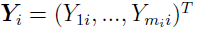 is sampled from a Gaussian distribution such that

where:
NSUB represents the number of subjects.
 is the multivariate Gaussian distribution with mean vector
  and the covariance matrix
  .
.
 is the function defining the PK/PD model.
 is a positive definite covariance matrix (
 ).
).
Note: This equation is another form of 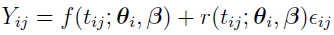 , discussed in the “Laplacian-Approximation-Based Algorithms” section, where replaces
  , and replaces the covariance part
 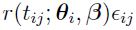 . It is used simply for notational convenience in this section.
Consider the case [3] 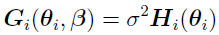 , where
  is a known function and =
  2. In this usage, a random effect parameter can change from subject to subject; while a fixed effect parameter is constant over the population.
Stage Two
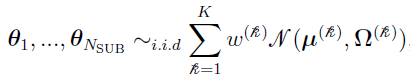
Each of the NSUB parameter vectors  is sampled from a Gaussian distribution with K mixing components:
(discussed in “Explore the Formulation of EM ”)
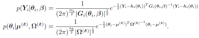
Given the observation  :
:
 can be defined as the likelihood function of
  given and .
 can be used to denote the multivariate Gaussian distribution of , with mean vector
  and covariance matrix
  .
.
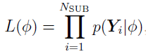
Now estimate  , which represents the collection of parameters
  , by maximizing the overall data likelihood L() which can be written as
where
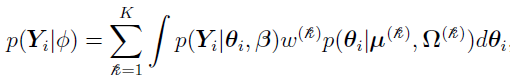
and the multivariate Gaussians are
This process is called the maximum likelihood estimate (MLE). The MLE of is defined as  such that
 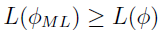 for all within the parameter space.