ADDL can be regarded as additional dose(s) that were not observed but were administered. For example, this can be used to indicate that additional doses will be given after the observed dose. Additional dose information needs to be provided and will be applied each time to the number of additional doses indicated by the ADDL record. Only numeric values or blanks are accepted in columns mapped to ADDL. A blank value is ignored.
When ADDL is checked in the Input Options tab (see the “Input Options tab” section), an ADDL column is added in the Main and Dosing mappings panels and an ADDL sub-menu for entering the additional dosing information is displayed in the tab. The information requested will be the Dosepoint (mode of administration and the name of the compartment in which the dose is administered), the Amount, the Rate if an infusion was administered, and Delta Time (i.e., the time interval between doses). The data structures for these options are the same as described in the steady-state section above. However, there is one major difference between ADDL and Steady State, even though the data structure requirements are the same. In Steady State, the dose occurs first, followed by the delta time; in ADDL, the delta time occurs first, followed by the dose.
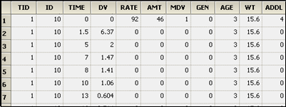
Example: The screen shot below is an ADDL set up to simulate a dosing regimen. For Subject ID 10, the simulated regimen consists of four infusions of 50 mass units at a rate of 100 mass units per time unit (i.e., duration=0.5 time units) every 72 time units (e.g., hours), starting at time zero.


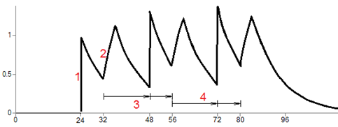
More complex example: Suppose a bolus dose of 1 unit given at time 24 (area 1 in the following graph), followed by a 4-time-unit infusion (area 2) started at time 32 (8 hours after the bolus), followed by two additional cycles (areas 3 and 4) just like it.

The additional cycles must start at the time of the last actual dose, which is the infusion that starts at time 32. The cycle, as depicted in area 3 for example, starts with an initial delay of 16 time units, then the bolus, then a delay of 8 time units, then the start of the next infusion. This cycle is repeated as many times as requested, in this case 2 times.
On the Input Options tab, check the ADDL option to display the ADDL sub-tab.
Press the Add button.
Notice how ADDL differs from the Steady-State user interface. The Delta Time delays come first.
Set up the first dosepoint:
a. Enter the initial delay (e.g., 16 time units).
b. Enter the name of the dose point to receive the dose (e.g., A1), if necessary.
c. Make sure the Bolus/Infusion option is set to Bolus.
d. Enter the amount of the dose (e.g., 1 unit).
Press the Add button.
Set up the second dosepoint.
a. Enter the initial delay (e.g., 8 time units).
b. Enter the name of the dosepoint (does not have to be the same as the prior dosepoint).
c. Make sure the Bolus/Infusion button says Infusion.
d. Enter the amount of the infusion (e.g., 1 unit).
e. With the Rate/Duration button displaying Rate and enter the rate (e.g., 0.25 drug units per time unit).
Note that the total cycle time is shown below the Add button.
The concentration-time curve shown in the previous graph arose from the following dosing input:

This says three things:
A simple bolus of 1 unit occurs at time 24.
A 4-time-unit infusion begins at time 32 (8 hours after the bolus).
Two of the ADDL cycles begin at time 32.
Since the first cycle begins with a 16-time-unit delay, it means that the bolus in the cycle occurs at time 48, which is 24 hours after the initial bolus called for in the data.
Specifying steady state and additional doses outside of the user interface
Steady state dosing can be specified outside of the user interface. Consider the following data from an input file.

The column definition text file contains these lines:
sscol(SS)
iicol(II)
ssoffcol(SSOffset)
where sscol(SS) indicates that there is a column named SS (meaning steady state), and iicol(II) indicates that there is a column named II (meaning interdose interval). The SS column contains values 1 or 2 (or nothing). Note, rows in which SS is 2 can only follow rows in which SS is 1 or 2.
When the first row is encountered, at time 0, it means that the model will undergo a cycle of II time units (in this case 8), where each iteration of the cycle consists of a dose of 100 to A1, and a dose of 30 to Aa, followed by 8 hours until the next repetition. This cycle is conceptually repeated sufficient times to bring the model to steady state, ending at time 0, because 0 is the time on the row. Then, at that time, the doses are repeated one more time.
Multiple cycles can be superimposed, as shown by the second row, in which SS is 2, indicating an 8 time-unit cycle with a dose of 50 to A1 and 60 to Aa. However, the doses are not given at time 0. They start at time 3, because there is a datum 3 in the SSOffset column. Therefore, the cycle looks like this:

Up to nine SS = 2 rows can follow an SS = 1 row. In addition, the interdose interval (II) values do not all have to be the same. However, the least common multiple of the interdose intervals must not be more than ten times the longest one. This prevents combinations of interdose intervals like 24 and 23 (for which the least common multiple would be 552 time units).
Note on transferring NONMEM datasets to NLME, and vice-versa: In the case that a NONMEM dataset contains rows in which SS = 2, and in which the time value on that row differs from the SS = 1 row above it, it is necessary to introduce an additional column for SSOffset:

Note the different values in the time column.

Note the same values in the time column with the additional offset column data (SSOffset).
This was necessitated by the Sort option on input data.
Additional doses can be specified as follows:

The column definition text file contains these lines:
addlcol(ADDL)
iicol(II)
where addlcol(ADDL) indicates that there is a column named ADDL (meaning additional), and iicol(II) indicates that there is a column named II (meaning interdose interval).
When the first row is encountered, at time 0, first the doses into A1 of 100 and Aa of 30 are performed, and then 10 more of those doses are scheduled into the future, at 8 time-unit intervals, because ADDL=10 and II=8.
Then, when the second row is encountered at time 3, first the doses into A1 of 50 and Aa of 60 are performed, and then 10 more of those doses are scheduled into the future, at 8 time-unit intervals.
Together the ADDL doses look like this:

SS and ADDL dosing may be combined, as in the following:

where the column definitions are:
sscol(SS)
iicol(II)
ssoffcol(SSOffset)
addlcol(ADDL)

Covariates may be included on SS or ADDL lines, but observations will be ignored.