All plot object except Scatter Plot, have a Graphs menu that lists all plots in the object. Many objects have plots with names based on the variables that are mapped to the X, Y, or Y2 contexts. For example, if Time is mapped to the X axis and Concentration is mapped to the Y axis, the plot is named Concentration vs Time.
Graphs menu options also change depending on whether or not a variable is mapped to the Y2 axis, multiple variables are mapped to the Y axis, Data Label, Group, or one of the Lattice Conditions contexts.
Y2: If a variable is mapped to the Y2 axis, then two plots are listed under Graphs. For example, if Time is mapped to the X axis and Effect is mapped to the Y2 axis, the second plot is named Effect vs Time.
Multiple Y: If more than one variable is mapped to the Y axis, then a separate plot for each mapped variable is listed under Graphs.
Data Label: If a variable is mapped the Data Label context and no variables are mapped to the Y2 axis or the Group contexts, then only one plot is listed under Graphs.
Group: If a variable is mapped to the Group context, then all variable values are listed under the plot name in the Graphs menu. For example, if Subject is mapped to the Group context, then all Subject identifiers are listed under the plot name. If multiple variables are mapped to the Group context to create unique profiles, then each profile is listed under the plot name.
Lattice Conditions: If a variable is mapped to one of the Lattice Conditions contexts and no variables are mapped to the Y2 axis or the Group contexts, then only one plot is listed under Graphs.
For Scatter Plots, there is no list of graphs, only a single Graph item that, when clicked, provides access to the Appearance tab for the plot.
Selecting a particular plot under the Graphs menu provides access to the following tabs of controls (tab and option availability depend on the plot type).
-
Content tab
Define data display and how quartiles and whiskers are generated
Set up histogram bins
Sort X values and specify offsets for multiple XY plots
Set up regression lines for XY plots
Set up error bars -
Appearance tab
Specify appearance of data labels
Specify appearance of bars
Specify appearance of borders
Specify appearance of markers
Specify appearance of data labels
Specify appearance of scatter plot diagonal labels
Specify appearance of lines
Specify appearance of error bars
Specify appearance for Group variables -
Quick Styles tab: quickly switch the XY plot between a line and a scatter plot and set Group options
Define data display and how quartiles and whiskers are generated
Select Graphs > <box graph name> in the tree, then click the Content tab.
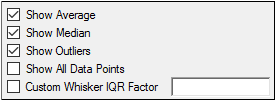
Use the Show Average checkbox to toggle display of the line indicating the average value of the data in the box plot.
Use the Show Median checkbox to toggle display of the line indicating the median value of the data in the box plot.
Use the Show Outliers checkbox to toggle display of the outliers in the plot display panel.
Use the Show All Data Points checkbox to toggle display of all data points in the plot display panel.
Check the Custom Whisker IQR Factor box to enter a custom value used to calculate the IQR (interquartile range).
In the Custom Whisker IQR Factor field, type the value to use as a multiplier used to determine how far to extend both the top and bottom whiskers.
Select Graphs > <histogram graph name> in the tree, then click the Content tab.
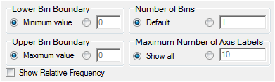
In the Lower Bin Boundary area, select Minimum value to use the lowest value of the variable mapped to the Distribution context as the minimum value, or select the option button beside the field and enter a value.
In the Upper Bin Boundary area, select Maximum value to use the highest value of the variable mapped to the Distribution context as the maximum value, or select the option button beside the field and enter a value.
In the Number of Bins area, select Default to use the default number of bins, or select the option button beside the field and enter the number of bins.
In the Maximum Number of Axis Labels area, select Show all to display all axis labels, or select the option button beside the field and type the maximum number of axis labels to display.
Check the Show Relative Frequency box to display the relative frequency on the Y axis. The default frequency display is a simple frequency.
Sort X values and specify offsets for multiple XY plots
Select Graphs > <graph name> in the tree, then click the Content tab.
These options are available for the output plots for the XY and X-Categorical XY Plot objects.
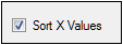
Graphs Options — Content tab for XY plots
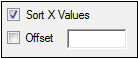
Offset option available for second and subsequent plots in a multi-plot graph
To control sorting of plots
Clear the Sort X Values checkbox to disable automatic sorting. When checked, the Sort X Values option sorts data in ascending X axis order before creating the plots. Clear this option when creating plots with a hysteresis curve.
To shift the first plot
For XY and X-Categorical XY Plot objects, when multiple columns are plotted on a single graph (e.g., predicted and observed results), each plot can be shifted to the left or right.
Shifting the first plot requires adjusting the X-axis range. Note that changing the range also affects the other plots, so it is recommended that you position the first plot, if desired, before setting the offsets for the other plots.
Select Axes > X in the tree, then click the Content tab.
Select the Custom option and adjust the values in the Minimum and Maximum fields.
To offset subsequent plots
Select the name of the plot to offset under the Graphs menu item.
On the Content tab check the Offset box and enter the number of units (for the XY Plot object) or pixels (for the X-Categorical XY Plot object) that the plot should be shifted. Entering a positive value moves the plot to the right, a negative value moves it to the left.
Set up regression lines for XY plots
Select Graphs > <XY graph name> > Regression in the tree, then click the Content tab.
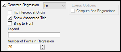
Check the Generate Regression box to display a regression line on the plot.
Select the type of regression line to display.
Ln (log base e)
Linear
LOESS (LOcally wEighted Scatter plot Smoothing)
If selected, the Loess Options group is made available
Note:If a regression line is selected, the values used to create the line are displayed across the top of the plot.
Ln: the log of the Y slope and the values of a and b.
Linear: The R-squared, intercept estimate, and slope estimate values are displayed.
LOESS: Nothing is displayed.
Select the Compute Abs Regressions checkbox to fit a LOESS regression to the absolute values of the dependent variable, in addition to the normal LOESS regression that does not take absolute values. The reflection of the absolute value fit through the X-axis is also included. This is useful when the magnitudes of the dependent variable are more important than the signed values, for example, weighted residuals.
Select the Fix Intercept at Origin checkbox to fix the intercept of a linear regression line at the plot’s origin. This option is only available when Linear regression is specified, as Ln and LOESS do not use intercept values.
Clear the Show Associated Title checkbox to not include the regression line equation in the title of the plot.
Check the Bring to Front checkbox to display the regression line in front of the data points.
In the Legend field, type a name for the regression line so it is displayed in the plot legend.
The Number of Points in Regression field controls the display of the regression line plot, by setting the number of points at which to evaluate and plot the regression line.
Special note for X-Categorical plots: For X-Categorical XY Plot objects, use the Descriptive Statistics object to compute data for the error bars. The Descriptive Statistics results worksheet will be used as input for a second plot, with the Mean column being mapped to the Y axis and the SD column mapped to the Error Bars context. Use the Offset option in the Content tab for the second plot to shift the error bars as desired. See the example “Multiple profile analysis using NCA”.
Select Graphs > <graph name> > Error Bars in the tree, then click the Content tab.
Error bars are available for an XY Plot, X-Categorical XY Plot, or a Column object that has no Group mapping.
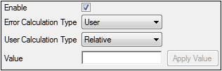
Clear the Enable checkbox to disable error bars. Check to enable, but additional mappings or settings are required before error bars will display.
In the Error Calculation Type menu, select the calculation type used to create the error bars.
FixedValue: Use the value entered in the Value field as the length of the lower and upper bars. Phoenix ignores the variable or variables mapped to the error bar contexts.
User: Apply the method selected in the User Calculation Type menu to the error bar mapped columns in the Data Mappings panel. Choose from:
Absolute: The mapped columns are Y-axis coordinates. Values mapped as Lower are the Y-axis coordinates for the ends of the lower error bars, and values mapped as Upper are the Y-axis coordinates for the ends of the upper error bars. The error bars display only when the mapped data values for Lower are below the corresponding plotted points or when the mapped data values for Upper are above the corresponding plotted points.
Relative: The mapped columns are error bar lengths. Values mapped as Lower are the lengths from the plotted points to the lower ends of the error bars, and values mapped as Upper are the lengths from the data points to the upper ends of the error bars.
Click Apply Value to use the typed value in the display of the error bars.
Specify appearance of data labels
For all plots except box plots, the display of labels for the data can be controlled. The background color for data labels can be set for scatter plots and grouped XY plots. Grouped XY plots also have a setting for the label color.
Select Graphs > <graph name> in the tree, then click the Appearance tab.
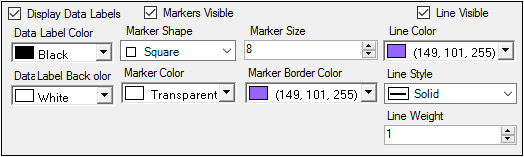
Check the Display Data Labels box to display variable values beside the bars/points.
In the Data Label Color menu, select the color for the data label by selecting a color scheme tab: Palette, Named, or System and clicking the color.
In the Data Label Back Color menu, select the background color for the data label by selecting a color scheme tab: Palette, Named, or System and clicking the color.
Bar appearance options are only available for Bar, Column, Box, and Histogram objects.
Select Graphs > <graph name> in the tree, then click the Appearance tab.
In the Bar Width box, select or type the width of the bars. (This option is only available for Bar and Column objects.)
In the Fill Color menu, select the color for the bar by selecting a color scheme tab: Palette, Named, or System and clicking the color.
Border appearance options are only available for Bar, Column, Box, and Histogram objects.
Select Graphs > <graph name> in the tree, then click the Appearance tab.
Select the color for the border by selecting a color scheme tab: Palette, Named, or System n the Border Color menu and clicking the color.
In the Border Style menu, select the style for the border.
In the Border Width box, select or type the width of the borders.
Marker appearance options are only available for Box, XY, QQ, Scatter Plot and X-Categorical XY Plot objects.
Select Graphs > <graph name> in the tree, then click the Appearance tab.
Check the Markers Visible box to display plot markers.
Select the shape to use as a data point marker from the Marker Shape menu.
In the Marker Color menu, select the color for the marker by selecting a color scheme tab: Palette, Named, or System and clicking the color.
In the Marker Size box, select or type the size of the data point markers.
In the Marker Border Color menu, select the color for the marker border by selecting a color scheme tab: Palette, Named, or System and clicking the color.
Specify appearance of data labels
Data label options are available for all plot objects except Box Plot objects.
Select Graphs > <graph name> in the tree, then click the Appearance tab.
Use the Display Data Labels checkbox to toggle the display of data point labels.
Turning on the checkbox adds the following two controls:
In the Data Label Color menu, select the color for the label by selecting a color scheme tab: Palette, Named, or System and clicking the color.
In the Data Label Back Color menu, select the background color for the label by selecting a color scheme tab: Palette, Named, or System and clicking the color.
Specify appearance of scatter plot diagonal labels
Diagonal labels are only applicable to Scatter Plot objects.
Select Graph in the tree.
In the Appearance tab, use the Display Diagonal Labels checkbox to toggle the display of labels along the diagonal.
Turning on the checkbox adds the Change Font button to the tab. Click to access tools for adjusting the label font, size, style, and effects.
The options described below can be used to change the appearance of lines in all groups by selecting the XY Plot or X-Categorical XY Plot in the tree. To only change the line appearance in an individual group, select that group in the tree.
To change the line display, click the plot node in the navigation tree. For regression lines, expand the plot node in the navigation tree and click Regression. If Compute Abs regressions is selected in the Regression Content tab, users can also format the LOESS absolute regression line display using the controls in the Abs Loess Lines area.
Select Graphs > <graph name> in the tree, then click the Appearance tab.
Check the Line Visible box to display a line connecting the points (this option is not available for regression lines).
In the Line Color menu, select the color for the line by selecting a color scheme tab: Palette, Named, or System and clicking the color.
In the Line Style menu, select the style for the line.
In the Line Weight box, select or type the weight of the line.
Specify appearance of error bars
Select Graphs > <graph name> in the tree, then click the Appearance tab.
Expand the plot node in the navigation tree and click Error Bars.
Click the Appearance tab.
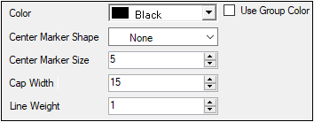
In the Color menu, choose the color used to display the error bars center point marker by selecting a color scheme tab: Palette, Named, or System and clicking the color.
Check the Use Group Color checkbox to use the Line Color specification in the plot’s Appearance tab to color the error bars.
In the Center Marker Shape menu, select the shape of the marker used to indicate the center point of the error bars. The default marker shape is None.
In the Center Marker Size field, type or use the arrows to change the size of the marker.
In the Cap Width field, type or use the arrows to change the width of the top and bottom bars.
In the Line Weight field, type or use the arrows to change the thickness of the error bar lines.
Specify appearance for Group variables
Several Plot objects contain a Group context. If one or more variables are mapped to the Group context, then the variable values are listed under Graphs > <graph name> in the tree.
Note:The plot object must be run before users can view Group variables in the Graphs menu.
Select a Group value to access its Appearance tab. The Group variables Appearance tab controls are the same as those in the XY plot Appearance tab (see “Specify appearance of data labels” and subsequent sections) with one extra field, Legend Text.
In the Legend Text field, type a label for the Group value in the legend.
The Quick Styles tab allows users to quickly switch the XY plot between a line and a scatter plot. Users can also use the tab to quickly update the plot display. The Quick Styles tab is only available in the XY Plot object.
Select Graphs > <graph name> in the tree, then click the Quick Styles tab.
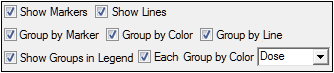
Options include:
Show Markers toggles display of markers. If at least one sort variable is mapped to the Group context, each profile is assigned its own unique marker shape and color combination, otherwise, all markers are the same by default. Clearing this option automatically clears the Group by Marker checkbox and all profiles are assigned the same marker shape.
Show Lines toggles displaying the plot as a line plot or as a scatter plot.
Group by Marker toggles displaying all markers as the same shape or by group. This option is only available when at least one variable is mapped to the Group context.
Group by Color toggles coloring all lines and markers the same (black by default) or by group. This option is only available when at least one variable is mapped to the Group context.
Group by Line toggles using the same style (solid by default) for all lines or style by group. This option is only available when at least one variable is mapped to the Group context.
Show Groups in Legend toggles the display of profiles in the plot legend. This option is only available when at least one variable is mapped to the Group context. Clearing this checkbox also clears and makes unavailable the Group by Marker, Group by Color, and the Group by Line checkboxes.
Each Group by Color toggles using the same color for each level (i.e., value) of the Group variable selected from the pull-down menu, when two or more variables are mapped to the Group context. Only the line color and the marker color will change, styles remain unchanged. If the user changes either a marker color or a line color for an individual member of the group (individual members are listed below Error Bars in the tree on the left), then that color change is applied to all the individuals members in the same group.
