Modeling and nonlinear regression
Model fitting algorithms and features of Phoenix WinNonlin
Modeling and nonlinear regression
The value of mathematical models is well recognized in all of the sciences — physical, biological, behavioral, and others. Models are used in the quantitative analysis of all types of observations or data, and with the power and availability of computers, mathematical models provide convenient and powerful ways of looking at data. Models can be used to help interpret data, to test hypotheses, and to predict future results. The main concern here is with “fitting” models to data — that is, finding a mathematical equation and a set of parameter values such that values predicted by the model are in some sense “close” to the observed values.
Most scientists have been exposed to linear models, models in which the dependent variable can be expressed as the sum of products of the independent variables and parameters. The simplest example is the equation of a line (simple linear regression):
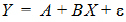
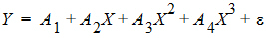
where Y is the dependent variable, X is the independent variable, A is the intercept and B is the slope. Two other common examples are polynomials such as:
and multiple linear regression.
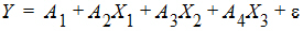
These examples are all “linear models” since the parameters appear only as coefficients of the independent variables.
In nonlinear models, at least one of the parameters appears as other than a coefficient. A simple example is the decay curve:
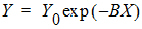
This model can be linearized by taking the logarithm of both sides, but as written it is nonlinear.
Another example is the Michaelis-Menten equation:
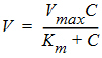
This example can also be linearized by writing it in terms of the inverses of V and C, but better estimates are obtained if the nonlinear form is used to model the observations (Endrenyi, ed. (1981), pages 304–305).
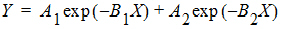
There are many models which cannot be made linear by transformation. One such model is the sum of two or more exponentials, such as:
All of the models on this page are called nonlinear models, or nonlinear regression models. Two good references for the topic of general nonlinear modeling are Draper and Smith (1981) and Beck and Arnold (1977). The books by Bard (1974), Ratkowsky (1983) and Bates and Watts (1988) give a more detailed discussion of the theory of nonlinear regression modeling. Modeling in the context of kinetic analysis and pharmacokinetics is discussed in Endrenyi, ed. (1981) and Gabrielsson and Weiner (2016).
All pharmacokinetic models derive from a set of basic differential equations. When the basic differential equations can be integrated to algebraic equations, it is most efficient to fit the data to the integrated equations. But it is also possible to fit data to the differential equations by numerical integration. Phoenix WinNonlin can be used to fit models defined in terms of algebraic equations and models defined in terms of differential equations as well as a combination of the two types of equations.
Given a model of the data, and a set of data, how is the model “fit” to the data? Some criterion of “best fit” is needed, and many have been suggested, but only two are much used. These are maximum likelihood and least squares. With certain assumptions about the error structure of the data (no random effects), the two are equivalent. A discussion of using nonlinear least squares to obtain maximum likelihood estimates can be found in Jennrich and Moore (1975). In least squares fitting, the “best” estimates are those which minimize the sum of the squared deviations between the observed values and the values predicted by the model.
The sum of squared deviations can be written in terms of the observations and the model. In the case of linear models, it is easy to compute the least squares estimates. One equates to zero the partial derivatives of the sum of squares with respect to the parameters. This gives a set of linear equations with the estimates as unknowns; well-known techniques can be used to solve these linear equations for the parameter estimates.
This method will not work for nonlinear models, because the system of equations which results by setting the partial derivatives to zero is a system of nonlinear equations for which there are no general methods for solving. Consequently, any method for computing the least squares estimates in a nonlinear model must be an iterative procedure. That is, initial estimates of the parameters are made and then, in some way, these initial estimates are modified to give better estimates, i.e., estimates which result in a smaller sum of squared deviations. The iteration continues until hopefully the minimum (or least) sum of squares is reached.
In the case of models with random effects, such as population PK/PD models, the more general method of maximum likelihood (ML) must be employed. In ML, the likelihood of the data is maximized with respect to the model parameters. The LinMix operational object fits models of this variety.
Since it is not possible to know exactly what the minimum is, some stopping rule must be given at which point it is assumed that the method has converged to the minimum sum of squares. A more complete discussion of the theory underlying nonlinear regression can be found in the books cited previously.
Model fitting algorithms and features of Phoenix WinNonlin
Phoenix WinNonlin estimates the parameters in a nonlinear model, using the information contained in a set of observations. Phoenix WinNonlin can also be used to simulate a model. That is, given a set of parameter values and a set of values of the independent variables in the model, Phoenix WinNonlin will compute values of the dependent variable and also estimate the variance-inflation factors for the estimated parameters.
A computer program such as Phoenix WinNonlin is only an aid or tool for the modeling process. As such it can only take the data and model supplied by the researcher and find a “best fit” of the model to the data. The program cannot determine the correctness of the model nor the value of any decisions or interpretations based on the model. The program does, however, provide some information about the “goodness of fit” of the model to the data and about how well the parameters are estimated.
It is assumed that the user of Phoenix WinNonlin has some knowledge of nonlinear regression such as contained in the references mentioned earlier. Phoenix WinNonlin provides the “least squares” estimates of the model parameters as discussed above. The program offers three algorithms for minimizing the sum of squared residuals: the simplex algorithm of Nelder and Mead (1965), the Gauss-Newton algorithm with the modification proposed by Hartley (1961), and a Levenberg-type modification of the Gauss-Newton algorithm (Davies and Whitting (1972)).
The simplex algorithm is a very powerful minimization routine; its usefulness has formerly been limited by the extensive amount of computation it requires. The power and speed of current computers make it a more attractive choice, especially for those problems where some of the parameters may not be well-defined by the data and the sum of squares surface is complicated in the region of the minimum. The simplex method does not require the solution of a set of equations in its search and does not use any knowledge of the curvature of the sum of squares surface. When the Nelder-Mead algorithm converges, Phoenix WinNonlin restarts the algorithm using the current estimates of the parameters as a “new” set of initial estimates and ting the step sizes to their original values. The parameter estimates which are obtained after the algorithm converges a second time are treated as the “final” estimates. This modification helps the algorithm locate the global minimum (as opposed to a local minimum) of the residual sum of squares for certain difficult estimation problems.
The Gauss-Newton algorithm uses a linear approximation to the model. As such it must solve a set of linear equations at each iteration. Much of the difficulty with this algorithm arises from singular or near-singular equations at some points in the parameter space.Phoenix WinNonlin avoids this difficulty by using singular value decomposition rather than matrix inversion to solve the system of linear equations. (See Kennedy and Gentle (1980).) One result of using this method is that the iterations do not get “hung up” at a singular point in the parameter space, but rather move on to points where the problem may be better defined. To speed convergence, Phoenix WinNonlin uses the modification to the Gauss-Newton method proposed by Hartley (1961) and others; with the additional requirement that at every iteration the sum of squares must decrease.
Many nonlinear estimation programs have found Hartley’s modification to be very useful. Beck and Arnold (1977) compare various least squares algorithms and conclude that the Box-Kanemasu method (almost identical to Hartley’s) is the best under many circumstances.
As indicated, the singular value decomposition algorithm will always find a solution to the system of linear equations. However, if the data contain very little information about one or more of the parameters, the adjusted parameter vector may be so far from the least squares solution that the linearization of the model is no longer valid. Then the minimization algorithm may fail due to any number of numerical problems. One way to avoid this is by using a ‘trust region’ solution; that is, a solution to the system of linear equations is not accepted unless it is sufficiently close to the parameter values at the current iteration. The Levenberg and Marquardt algorithms are examples of ‘trust region’ methods.
Note:The Gauss-Newton method with the Levenberg modification is the default estimation method used by Phoenix WinNonlin.
Trust region methods tend to be very robust against ill-conditioned data sets. There are two reasons, however, why one may not want to use them. (1) They require more computation, and thus are not efficient with data sets and models that readily permit precise estimation of the parameters. (2) More importantly, the trust region methods obtain parameter estimates that are often meaningless because of their large variances. Although Phoenix WinNonlin gives indications of this, it is possible for users to ignore this information and use the estimates as though they were really valid. For more information on trust region methods, see Gill, Murray and Wright (1981) or Davies and Whitting (1972).
In Phoenix WinNonlin, the partial derivatives required by the Gauss-Newton algorithm are approximated by difference equations. There is little, if any, evidence that any nonlinear estimation problem is better or more easily solved by the use of the exact partial derivatives.
To fit those models that are defined by systems of differential equations, the RKF45 numerical integration algorithm is used (Shampine, Watts and Davenport (1976)). This algorithm is a 5th order Runge-Kutta method with variable step sizes. It is often desirable to set limits on the admissible parameter space; this results in “constrained optimization.” For example, the model may contain a parameter which must be non-negative, but the data set may contain so much error that the actual least squares estimate is negative. In such a case, it may be preferable to give up some of the properties of the unconstrained estimation in order to obtain parameter estimates that are physically realistic. At other times, setting reasonable limits on the parameter may prevent the algorithm from wandering off and getting lost. For this reason, it is recommend that users always set limits on the parameters (the means of doing this is discussed in “Parameter Estimates and Boundaries Rules” and “Modeling”). In Phoenix WinNonlin, two different methods are used for bounding the parameter space. When the simplex method is used, points outside the bounds are assigned a very large value for the residual sum of squares. This sends the algorithm back into the admissible parameter space.
With the Gauss-Newton algorithms, two successive transformations are used to affect the bounding of the parameter space. The first transformation is from the bounded space as defined by the input limits to the unit hypercube. The second transformation uses the inverse of the normal probability function to go to an infinite parameter space. This method of bounding the parameter space has worked extremely well with a large variety of models and data sets.
Bounding the parameter space in this way is, in effect, a transformation of the parameter space. It is well known that a reparameterization of the parameters will often make a problem more tractable. (See Draper and Smith (1981) or Ratkowsky (1983) for discussions of reparameterization.) When encountering a difficult estimation problem, the user may want to try different bounds to see if the estimation is improved. It must be pointed out that it may be possible to make the problem worse with this kind of transformation of the parameter space. However, experience suggests that this will rarely occur. Reparameterization to make the models more linear also may help.
Because of the flexibility and generality of Phoenix WinNonlin, and the complexity of nonlinear estimation, a great many options and specifications may be supplied to the program. In an attempt to make Phoenix WinNonlin easy to use, many of the most commonly used options have been internally specified as defaults.
Phoenix WinNonlin is capable of estimating the parameters in a very large class of nonlinear models. Fitting pharmacokinetic and pharmacodynamic models is a special case of nonlinear estimation, but it is important enough that Phoenix WinNonlin is supplied with a library of the most commonly used pharmacokinetic and pharmacodynamic models. To speed execution time, the main Phoenix WinNonlin library has been built-in, or compiled. However, ASCII library files corresponding to the same models as the built-in models, plus an additional utility library of models, are also provided.
