Linear mixed effects model examples
Knowledge of how to do basic tasks using the Phoenix interface, such as creating a project and importing data, is assumed.
Analyzing treatment effects
Analyzing variance structure effects
This example uses the Linear Mixed Effects (LinMix) capability in Phoenix to test for differences among treatment groups in a parallel study. Twenty-eight subjects were randomly assigned to four treatment groups. One observation of drug effect was measured from each subject for a total of seven observations per treatment. If statistically significant differences are observed between treatments, then the estimates, with intervals, are desired.
The model for these data is as follows.
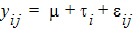
where:
i is the treatment index, 1, 2, 3, 4
j is the subject index within treatment, 1, 2, …, 7
yij is the observation value for treatment i, subject j
m is the overall mean
ti is the effect of treatment i
eij is the random error term for observation yij
Note:The completed project (LinMix_TreatmentEffects.phxproj) is available for reference in …\Examples\WinNonlin.
-
Create a new project with the name LinMix_TreatmentEffects.
-
Import the file …\Examples\WinNonlin\Supporting files\OneWayData.CSV.
-
Right-click OneWayData in the Data folder and select Send To > Computation Tools > Linear Mixed Effects.
-
In the Main Mappings panel:
Map Treatment to the Classification context.
Map Response to the Dependent context. -
In the Fixed Effects tab below the Setup panel, drag Treatment from the Classification list up to the Model Specification field (or type Treatment in the Model Specification field).
-
None is selected by default in the Dependent Variables Transformation menu. Do not change this setting.
-
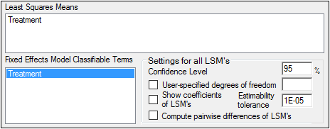
Select the Least Squares Means tab.
-
Drag Treatment from the Fixed Effects Model Classifiable Terms list to the Least Squares Means field.
Execute and evaluate the results
-
Click
 (Execute icon) to execute the object.
 -
Select Final Fixed Parameters in the Results list.
This model is over parameterized. There are five parameters, m, t1, t2, t3, t4, but there are only four means. The last parameter is removed from the model and is not estimated, resulting in the output of “Not estimable” for the Placebo group. When that happens, each of the other t parameters represents the difference between the treatment mean and the last treatment mean. Note that subtracting the Least Squares Means for high dose group from the mean for placebo produces the same number as t1. The parameter m is then the mean of the omitted treatment group, the placebo group in this case. -
Select Least Squares Means in the Results list.
On the Least Squares Means (LSM) tab, Estimate, for balanced data, is the average of the observations within each treatment group. Also listed are the standard error of each mean, p value for the hypothesis that the true mean equals zero, and interval. -
Select Partial Tests in the Results list.
In this case, the partial tests have the same value as the sequential test. This is always true for balanced datasets. For unbalanced data, these results can differ. Refer to “Least squares means” for more information on unbalanced data. -
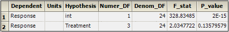
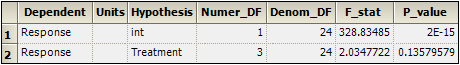
Select Sequential Tests in the Results list.
The p-value is shown as 0.1358, indicating that differences among treatment groups were not statistically significant.
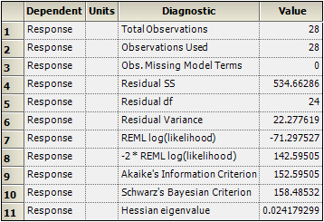
The Diagnostics results worksheet is opened by default in the Results tab.
This concludes the LinMix treatment effects analysis example.
Analyzing variance structure effects
This analysis is concerned with the precision components of assay validation to estimate contributions due to assay variation, assay-to-assay variation, and analyst-to-analyst variation. A single QC sample was prepared containing, theoretically, 65 ng/mL of analyte. Five analysts were recruited for this study. Each analyst ran five aliquots of the sample on four assay runs. The data are available in the dataset AssayVal1.CSV in the Phoenix examples directory.
Note:The completed project (LinMix_StructureEffects.phxproj) is available for reference in …\Examples\WinNonlin.
Set up the object
-
Create a project called LinMix_StructureEffects.
-
Import the file …\Examples\WinNonlin\Supporting files\AssayVal1.CSV.
Units must be added to the Determination column before the dataset can be used in a Linear Mixed Effects model. -
In the Columns tab below the table, select the Determination column header in the Columns list.
-
Clear the Unit field, type ng/mL, and press the Enter key.
-
Right-click Workflow in the Object Browser and select New > Computation Tools > Linear Mixed Effects.
-
Drag the AssayVal1 worksheet from the Data folder to the Main Mappings panel.
Map Analyst to the Classification context.
Map Assay to the Classification context.
Map Determination to the Dependent context. -
Select the Variance Structure tab below the Setup panel.
-
Drag Analyst from the Classification Variables list to the Random Effects Model field in the Random 1 sub-tab (or type Analyst in the field).
-
Click Add Random to add another Random effect.
-
Drag Assay from the Classification Variables list to the Random Effects Model field in the Random 2 sub-tab (or type Assay in the field).
-
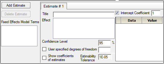
Select the Estimates tab.
-
Check the Intercept Coefficient checkbox and type 1 in the Intercept Coefficient field.
Execute and view the results of the first model
-
Execute the object.
-
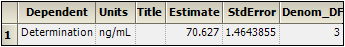
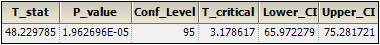
Select Estimates in the Results list.
Statistical accuracy values are located in the Estimates worksheet. The mean response is the intercept, which is estimated at 70.6 ng/mL with a 95% confidence interval. The lower interval is 65.97 and the upper interval is 75.28. Since the theoretical analyte concentration of 65 ng/mL is not within the interval, one can conclude that the bias is statistically significant. The method has a bias of approximately 5 ng/mL. -
Select the Final Variance Parameters worksheet to view precision estimates and variance components.
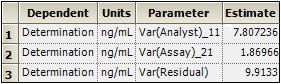
Based on these results, most of the variation is coming from analyst-to-analyst variation and from within-assay variation. Assay-to-assay noise is quite small. The units on the variances are (ng/mL).
Apply model to a different dataset
Now fit the same model to the data in the dataset AV3.CSV.
-
Import the file …\Examples\WinNonlin\Supporting files\AV3.CSV.
Units must be added to the Determination column before the dataset can be used in a Linear Mixed Effects model. -
In the Columns tab, select the Determination column header in the Columns box.
-
Clear the Unit field, type ng/mL, and press the Enter key.
-
Right-click the Linear Mixed Effects object in the Object Browser and select Copy.
-
Right-click Workflow and select Paste.
A new Linear Mixed Effects object named Copy of Linear Mixed Effects is added to the Workflow. The LinMix object copy contains the same settings as the original object. -
Map the AV3 dataset to Copy of Linear Mixed Effects. Do not change the data mappings in the Main Mappings panel.
Execute and view the results from the second model
-
Execute the object.
-
Select Final Variance Parameters in the Results list.
The Final Variance Parameters worksheet contains the following variance components: -
In the Results tab, select the Warnings and Errors text file.
The text file states: “Warning 11094: Negative final variance component. Consider omitting this VC structure.” Problems associated with a linear mixed effects model are written to this file during execution.
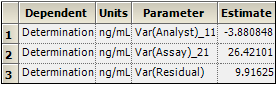
This table indicates that analyst-to-analyst variation is negative. Since variances cannot be negative, it is customary to replace the value with zero. A negative variance component indicates that the corresponding term should be removed from the model, which means that the contribution from that term is minimal compared to the contribution due to the other terms and it cannot be distinguished from the residual term.
From the variance components it is clear that the largest contribution to noise in the method is from run-to-run variation. Within-run variation also contributes to the noise. There is very little variation among analysts, indicating that the method is robust.
The Linear Mixed Effects object warns user about negative final variances.
This concludes the LinMix structure effects analysis example.
