Levy plots compare InVivo absorption and InVitro dissolution data visually, as time-versus-time plots at matched values for absorption and dissolution. The plots include a linear fit of the data points with intersection at origin, and the correlation (R2) value and the slope for the model line, as well as a line at unity.
Levy plots require two separate datasets, one containing InVivo and the other containing InVitro data. Phoenix uses these datasets to plot InVivo versus InVitro times at user-specified Y values (typically, fraction absorbed or dissolved), using linear interpolation to calculate data points as needed. Matched time pairs are sampled from the data within the range from zero to the maximum observed dissolution or deconvolved absorption value, whichever is smaller.
The InVivo and InVitro datasets can contain the same or different sort variables. If sort variables with identical column names are in both datasets, then Phoenix includes only the sorting values that exist in both datasets. For non-matching sort variables, Phoenix uses the cross-product of the sort values to create the plots.
If units are used with the dataset variables mapped to the Values contexts, then the units must match in the InVivo and InVitro datasets.
The Levy Plot object groups data by formulation for each plot. Each formulation is displayed in a different color and is listed in the plot legend. The Levy Plot object uses only those formulation values that are in both datasets.
If a Y value to be plotted exists in the dataset, Phoenix uses the data. Otherwise, all other values are computed using simple linear interpolation. Data for formulation values that exist in only one dataset are not displayed in the plot or worksheet output. If no formulation values match in either dataset, then no output is created.
Note:The summary line on each Levy plot is fit to all matching formulations.
Use one of the following to add the object to a Workflow:
Right-click menu for a Workflow object: New > IVIVC > LevyPlot.
Main menu: Insert > IVIVC > Levy Plot.
Right-click menu for a worksheet: Send To > IVIVC > LevyPlot.
Note:To view the object in its own window, select it in the Object Browser and double-click it or press ENTER. All instructions for setting up and execution are the same whether the object is viewed in its own window or in Phoenix view.
This section contains the following topics:
InVitro and InVivo panels
Match Values panel
Options tab
Plots tab
Results
Use the Main Mappings panel to identify how input variables are used in a LevyPlot object. Required input is highlighted orange in the interface.
None: Data types mapped to this context are not included in any analysis or output.
Sort: Individual profiles used to sort the output into separate plots.
Independent: Sampling time values.
Values: Concentration sampling values, one value per sampling time per profile (see note below). Values from both datasets must have the same units.
Formulation: Drug formulation identifiers. Blank/empty formulation cells are not supported.
Caution:If the datasets both have a column named “Formulation,” these two columns will be used, even if they are not mapped in the panels. The Levy Plot will fail if the values in the two columns do not match.
Note:In cases where a profile has more than one value for a time point, use Descriptive Statistics on the source workbooks to average the values for each profile so that there is one value per time point. Then execute the Levy Plots object on the two Descriptive Statistics output.
Required input is highlighted orange in the interface.
None: Data types mapped to this context are not included in any analysis or output.
Formulation: Formulation data.
Interpolation Values: Interpolation values used to plot InVivo and InVitro time values at specified intervals.
Additional notes on match values
The Levy Plot object plots InVivo versus InVitro times corresponding to the Y values selected in the InVivo and InVitro panels. Match values are applied to all sort profiles, so there can be no missing or null values in the sort keys or an error is generated. The default interpolation values are zero to one, incremented by 0.1 for each sort profile. Users can also enter their own Y values to plot interpolated times using those values.
The InVivo dataset sampling time values are used for the Y-axis data. The match values must match the time units used in the InVivo dataset. For example, if sampling time is measured in hours, then the match values must correspond to the hourly sampling times. If sampling time is measured in days, then match values must correspond to the daily sampling times.
If an internal worksheet is used, the match values are applied to all profiles. If an external worksheet is used, users can map formulation data that uses different matched values for different formulations.
-
In the Levy Plots, the first value is displayed at Y=0, then at the specified interval up to the end of the sample data range. For example, an interval value of 10 generates plot values at Y=0, 10, 20, 30, etc. for the sampling time input data.
-
If the same values are entered for each profile, then interpolated time values are plotted at regular intervals across the sample data.
The maximum Y value displayed in the plot is the lesser of the maximum observed fraction dissolved and the calculated fraction absorbed. The Levy Plot object does not plot any points that are extrapolated from one of the datasets.
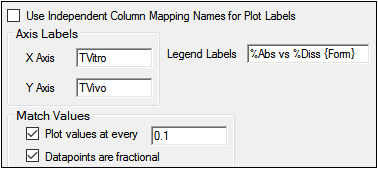
The Options tab allows users to specify how plot labels are displayed.
-
Check the Use Independent Column Mappings Names for Plot Labels checkbox to use the dataset variables mapped to the Independent contexts in the InVivo and InVitro panels as the plot labels.
-
In the Axis Labels area, enter any custom labels for the axes and legend.
•In the X Axis field, type a custom X-axis label.
•In the Y Axis field, type a custom Y-axis label.
•In the Legend Labels field, type a custom label for the plot legends.
-
In the Match Values area, specify interpolated time value intervals and whether or not the independent variable is fractional or a decimal.
The Plot Values at every checkbox is selected by default. This option creates a plot of interpolated time values at regular intervals across the sample data.
Enter the interval value in the Plot Values at every field, or leave the default value. The first value is displayed at Y=0, then at the specified interval until the end of the sample data range. For example, an interval value of 10 generates plot values at Y=0, 10, 20, 30, and so forth until the end of the data range is reached. The maximum Y value displayed is the lesser of the maximum observed fraction dissolved and the calculated fraction absorbed.
The Datapoints are fractional checkbox is selected by default. Leave this option selected if the data are expressed as fractions instead of percentages. Phoenix multiplies the values by 100 before plotting.
Note:To enter interpolation values manually, clear the Plot values at every checkbox in the Options tab, select a cell in the Values column (in the Mappings panel) and type the interpolation value. Continue selecting cells and entering values until all of the desired interpolation values are entered.
See the Plots tab description in the Loo Riegelman section.
The Levy Plot object creates one text file, one plot or group of plots, and two worksheets in the Results tab. The plot panel displays one levy plot for each individual profile.
Worksheet
-
Levy Plot Values: Values used in the plots, including interpolated and original data values, where interpolation was not necessary, including any sort variables. For each unique combination of sort variable values, the plot output contains Formulation data, if included, Values, TVitro, and TVivo.
-
Parameters: Output from fitting model 502, including estimates and statistics for the Y-intercept (INT) and slope.
Text File
-
Settings: User-defined settings.
Note:Word Export is not recommended for Levy Plots as the export would include all internal/hidden steps whose results are not readily discernible to the user.
Users can double-click a plot in the Results tab to edit it. (See the menu options descriptions in the Plots chapter of the Data Tools and Plots Guide for plot editing options.)
The default for the regression line in the Levy Plot is to fix the intercept at the origin. To calculate the intercept, do the following steps:
-
From the Results tab, double-click the Levy Plot to display it as a separate window.
-
In the tree view, select Graphs > Levy Plot > Regression.
-
Clear the Fix intercept at origin checkbox.
