Example - Bioequivalence

Bioequivalence model examples

Knowledge of how to do basic tasks using the Phoenix interface, such as creating a project and importing data, is assumed.

Analyzing average bioequivalence of 2x2 crossover study example
Analyzing average bioequivalence of a replicated crossover design example
Evaluating individual and population bioequivalence example

Analyzing average bioequivalence of 2x2 crossover study example

The objective of this study is to compare a newly developed tablet formulation to the capsule formulation that was being used in Phase II studies. Both had a label claim of 25 mg per dosing unit.

A 2x2 crossover design was chosen for this study. Twenty subjects were randomly assigned to one of two sequence groups. Within each sequence group, each subject took both formulations, with a washout period between. Drug concentrations in plasma were measured, and the AUClast (area under a curve computed to the last observation) was calculated.

Data for this example are provided in …\Examples\WinNonlin\Supporting files. The dataset used is Data 2x2.CSV.

The completed project (Bioequivalence_2x2.phxproj) is available for reference in …\Examples\WinNonlin.

Set up the object

Create a new project named Bioequivalence_2x2.
Import the file …\Examples\WinNonlin\Supporting files\Data 2x2.CSV.
Right-click Data 2x2 in the Data folder and then select Send To > Computation Tools > Bioequivalence.
In the Main Mappings panel:
Leave Sequence mapped to the Sequence context.
Leave Subject mapped to the Subject context.
Leave Period mapped to the Period context.
Leave Formulation mapped to the Formulation context.
Map AUClast to the Dependent context.
In the Model tab below the Setup panel, make sure that:
Crossover is selected as the Type of study,
Average is selected as the Type of Bioequivalence, and
Capsule is selected as the Reference Formulation.
Select the Fixed Effects tab, make sure that:
Sequence+Formulation+Period appears in the Model Specification field.
Ln(x) is selected in the Dependent Variables Transformation menu.
Select the Variance Structure tab.

The random effects are already specified in the Variance Structure tab. If they are not, type Subject(Sequence) in the Random Effects Model field.

Execute and view the results

Click (Execute icon) to execute the object.

The Average Bioequivalence worksheet indicates that the difference in ln(AUClast) between formulations is 0.046±0.073 (Difference±Diff_SE). The 90% confidence interval for the ratio is 92.216 (CI_90_Lower) to 118.780 (CI_90_Upper).

Since the interval is completely contained between 80 and 125, one can conclude that the formulations are bioequivalent.
Select the Partial Tests worksheet and compare with the Sequential Tests worksheet.

Because the data are balanced, the sequential and partial tests are identical. Note that, in the tests, Sequence is statistically significant, but no other factor is.

Select any cell with a numerical value in the Bioequivalence worksheet output and look in the value display bar above to see the full precision of 15 decimal places.

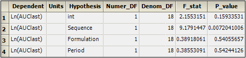
Sequential Tests worksheet for 2x2 crossover study

This concludes the Bioequivalence example of analyzing a 2x2 crossover study.

Analyzing average bioequivalence of a replicated crossover design example

The objective of this study is to compare a newly developed tablet formulation to a capsule formulation that was used in Phase II studies. Both formulations have the same label claim per dosing unit.

A RTRT/TRTR replicated crossover design was chosen for this study. Twenty subjects were randomly assigned to one of two sequence groups. Concentrations of the drug were measured in plasma, and the AUClast (area under the time-concentration curve, computed to the last observation) was calculated.

Note:The completed project (Bioequivalence_replicated.phxproj) is available for reference in …\Examples\WinNonlin.

Set up the object

Create a project called Bioequivalence_replicated.
Import the file …\Examples\WinNonlin\Supporting files\Data 2x4.CSV.

Right-click Data 2x4 in the Data folder and select Send To > Computation Tools > Bioequivalence.
In the Mappings panel:
Leave Sequence mapped to the Sequence context.
Leave Subject mapped to the Subject context.
Leave Period mapped to the Period context.
Leave Formulation mapped to the Formulation context.
Map AUClast to the Dependent context.
In the Model tab below the Setup panel, make sure that:
Crossover is selected as the Type of study,
Average is selected as the Type of Bioequivalence, and
Capsule is selected as the Reference Formulation.
Select the Fixed Effects tab and make sure that:
Sequence+Formulation+Period appears in the Model Specification field.
Ln(x) is selected in the Dependent Variables Transformation menu.

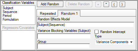
Note:Phoenix has automatically selected a model specification and classification variables based on the model for replicated crossovers.

Select the Variance Structure tab.

Notice that the default variance structure for a replicated crossover design is substantially different from and more complex than that for the 2x2 crossover design. As a result, the model fitting is more difficult as well.

In the Random 1 sub-tab, make sure that:
Formulation appears in the Random Effects Model field.
Subject appears in the Variance Blocking Variables field.
Banded No-Diagonal Factor Analytic(f) is selected in the Type menu.
2 is specified as the Number of factors.

In the Repeated sub-tab, make sure that:
Period appears in the Repeated Specification field.
Subject appears in the Variance Blocking Variables field.
Formulation appears in the Group field.
Variance Components is selected in the Type menu.

Execute and view the results

A user can expect that about 50% of datasets analyzed will produce a non-positive definite G matrix. This does not imply that the model-fitting is invalid, but only that a user must be careful not to over-interpret the variance estimates. The interval on the formulation difference will still have the expected statistical properties.

Execute the object.

The Average Bioequivalence worksheet indicates that the analysis just failed to show bioequivalence since the 90% confidence interval=91.612 (CI_90_Lower) and 125.772 (CI_90_Upper).
Select the Partial Tests worksheet and compare with the Sequential Tests worksheet.

Because the data are balanced, the sequential and partial tests are identical.

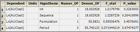
Partial Tests worksheet for replicated crossover study

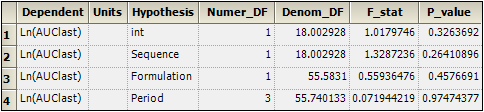
Sequential Tests worksheet for replicated crossover study

This concludes the Bioequivalence example of analyzing a replicated crossover study.

Evaluating individual and population bioequivalence example

Phoenix can handle a wide variety of model designs suitable for assessing individual and population bioequivalence, including:

TRTR/RTRT/TRRT/RTTR
TT/RR/TR/RT
TRT/RTR/TRR/RTT
TRRTT/RTTRR
TRR/RTR/RRT
RTR/TRT
TRR/RTT/TRT/RTR/TTR/RRT
TRRR/RTTT
TTRR/RRTT/TRRT/RTTR/TRRR/RTTT

where T=Test formulation and R=Reference formulation.

Note:Each sequence must contain the same number of periods. For each period, each subject must have one measurement.

A bioequivalence example, included as part of “Testing the Phoenix installation”, shows results for a RTR/TRT design. This example demonstrates an analysis of a TT/RR/TR/RT design.

Note:The completed project (Bioequivalence_IndPop.phxproj) is available for reference in …\Examples\WinNonlin.

Set up the population/individual model

Create a project called Bioequivalence_IndPop.
Import the file …\Examples\WinNonlin\Supporting files\TT RR RT TR.DAT.

Notice that the number of subjects is not the same in each sequence group. TT, RR, TR, and RT each have 4 subjects, whereas RT has 5.
Right-click TT RR RT TR in the Data folder and select Send To > Computation Tools > Bioequivalence.
In the Model tab below the Setup panel, select the Population/Individual option button in the Type of Bioequivalence area.
Map the data types to the following contexts:
Leave Sequence mapped to the Sequence context.
Leave Subject mapped to the Subject context.
Leave Period mapped to the Period context.
Leave Formulation mapped to the Formulation context.
Map AUC to the Dependent context.
In the Model tab, make sure that:
Crossover is selected in the Type of study area. Crossover studies are the only permitted type for Population/Individual bioequivalence analysis.
Population/Individual is set as the Type of Bioequivalence.
R is selected in the Reference Value menu.
Select the Fixed Effects tab and make sure that Ln(x) is set as the Dependent Variables Transformation. The values will be log-transformed before the analysis.
Select the Options tab and enter 95 as the Confidence Level.

Execute and view the Population/Individual model results

Execute the object.
Select the Population Individual worksheet in the Results list.

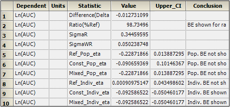
Inspect the results for mixed scaling. For population bioequivalence, the upper limit is 0.014 > 0, and therefore population BE has not been shown. For individual bioequivalence, the upper limit is –0.05 < 0, and so individual BE has been shown.

Compare average bioequivalence

Right-click the Bioequivalence object in the Object Browser and select Copy
Right-click Workflow in the Object Browser and select Paste.
In the Model tab of the copied object, select Average as the Type of Bioequivalence and make sure that:
Crossover is selected as the Type of study, and
R is selected as the Reference Formulation.
Select the Fixed Effects tab and make sure that:
Sequence+Formulation+Period appears in the Model Specification field.
Ln(x) is selected in the Dependent Variables Transformation menu.
Select the Variance Structure tab.

In the Random 1 sub-tab, make sure that:
Formulation appears in the Random Effects Model field.
Subject appears in the Variance Blocking Variables field.
Banded No-Diagonal Factor Analytic(f) is selected in the Type menu.
2 is in the Number of factors field.

Select the Variance Structure’s Repeated tab and make sure that:
Period appears in the Repeated Specification field.
Subject appears in the Variance Blocking Variables field.
Formulation appears in the Group field.

Execute and view the average bioequivalence results

Execute the object.

Using the model for average bioequivalence on replicated crossover designs resulted in a 90% lower interval of 87.277% (CI_90_Lower) and a 99.715% upper interval (CI_90_Upper) for the ratio of average AUC. Therefore a user can also conclude average bioequivalence is achieved. This is not always the case. Data can pass individual BE and fail average BE, and data can also pass average BE and fail individual BE.

This concludes the Bioequivalence individual/population evaluation example.