Testing the Phoenix installation
The following instructions test the installation of Phoenix WinNonlin by using a number of the sample files provided with the software. This chapter is not intended as a full validation of the product. It is intended to test for proper installation of major components of the application.
A set of Validation Suite Products is available from Certara. Contact the Certara sales department for more information.
Start Phoenix and create a new project
-
Double-click the Phoenix icon (
 ) on your desktop to start Phoenix.
 -
Select File > New Project to create a new project. A new project is created in the Object Browser.
-
Name the new project Install Test.
Note:AutoPilot users running on 64-bit operating systems should run the 32-bit version of Phoenix (Phoenix32) as opposed to the 64-bit version. The Phoenix desktop icon should be updated to reference the Phoenix32 executable as well.
The left panel’s default view is the Object Browser, which contains the project, and the other folders and objects that are contained in the project. The right viewing panel’s default view is blank, unless one of the project folders or the workflow is selected.
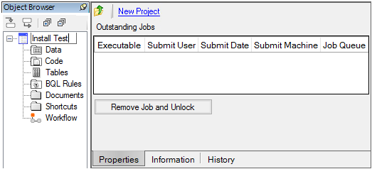
Creation of Install Test project denotes successful installation test
Confirm license installation
The ability to execute different Phoenix plug-ins depends on the license type installed. Use the Preferences dialog to check the installed Phoenix license(s).
-
Select Edit > Preferences to access the Preferences dialog.
-
Select Licensing > License Management to access the list of available licenses.
-
Confirm that the purchased license or licenses are listed in the Licenses panel.
Confirm plug-in startup
The Phoenix architecture is based on a series of plug-ins that allow different features to be enabled or disabled. Phoenix initializes these plug-ins when the application starts. The default setting is for all plug-ins to initialize when Phoenix starts. The plug-in initialization is independent of the installed license(s).
-
In the Preferences dialog, click Plugins to view the list of available plug-ins.
-
Select the General, System, and Non-loaded tabs to see the review the state of each plug-in type and to confirm they are started.
-
Click OK to exit the Preferences dialog.
•The Plugins panel on the right contains three tabs: General, System, and Non-loaded.
•Each plug-in has two possible states, Started and Stopped.
•All plug-ins are started the first time Phoenix is started.
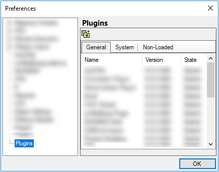
Plugins Preferences panel
Import a dataset
The dataset Bguide1.dat is used to test key Phoenix functions.
-
Select File > Import, click
 (Import File icon), or right-click the Data Folder in the Object Browser and select Import to display the Import File(s) dialog.
 -
Navigate to <Phoenix_install_dir>\application\Examples\WinNonlin\Supporting files).
-
Select the file Bguide1.dat and click Open.
The File Import Wizard dialog is displayed. The dialog is used to assign options for how the data are imported and presented. -
Click Finish. The dataset is added to the project Data folder and the worksheet is displayed in the right viewing panel.
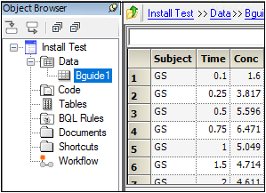
View of a dataset
Create a plot
-
Select the Workflow object in the Object Browser and then select Insert > Plotting > XY Plot.
Or
Right-click the Workflow object and select New > Plotting > XY Plot.
The XY Plot object is added to the workflow in the Object Browser and is automatically opened in the right viewing panel. The default view of an object is the Setup tab, which contains all the steps necessary to set up an object. -
Use the pointer to drag the Bguide1 worksheet from the Data folder to the XY Data Mappings panel.
-
Use the option buttons in the XY Data Mappings panel to map the data types to the following contexts:
Map Subject to the Group context.
Map Time to the X context.
Map Conc to the Y context. -
Click
 (Execute icon) to execute the workflow.
 -
Now use the Bguide1 dataset to test the Table object and its summary statistics function.
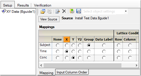
Context mapping for XY Plot
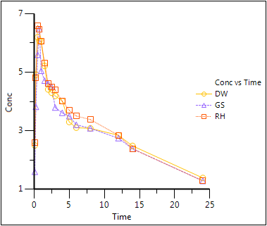
XY Plot results
Create a table
-
Add the Table object to the workflow by selecting the Workflow object in the Object Browser and then selecting Insert > Reporting > Table.
-
Map the dataset Bguide1 as the input source for the Table object by dragging the Bguide1 worksheet from the Data folder to the Table object Main Mappings panel.
-
Use the option buttons in the Main Mappings panel to map the data types to the following contexts:
Map Subject to the Stratification Row context.
Leave Time mapped to None.
Map Conc to the Data context. -
In the Options tab (located below the Setup tab, specify which table type the Table object is to use by selecting Table 1 - Column Summary by Row Stratification from the Table Type menu.
-
Select the Page Break on Row Stratification checkbox.
-
Select the Statistics tab, which is located underneath the Setup tab.
-
Click Select All to select all output statistics.
-
Execute the object.
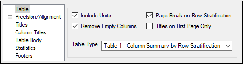
Setting Table object options
The results are presented as three HTML tables in the Results tab. Compare the tables in the Results tab to the tables pictured below.
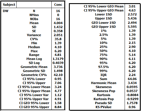
Resulting HTML table for subject DW
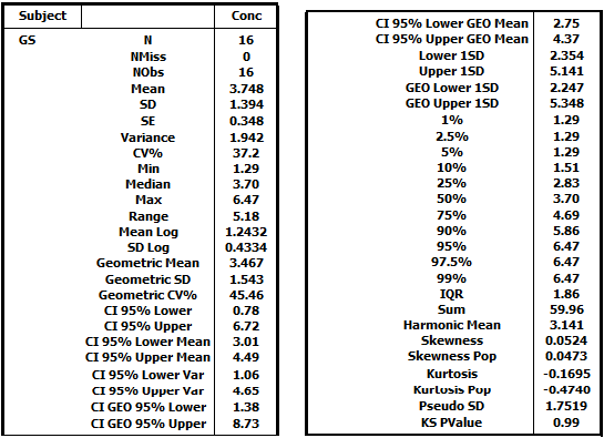
Resulting HTML table for subject GS
Resulting HTML table for subject RH
Confirm noncompartmental analysis functions
-
Select File > Load Project. The Load Project dialog is displayed.
-
Navigate to <Phoenix_install_dir>\application\Examples\WinNonlin.
-
Select Multiple_Profiles.phxproj and click Open.
This project contains: -
Expand the workflow node.
-
Select the NCA model object in the Object Browser.
-
Select items in the Setup tab list to explore the data mappings and option settings.
-
Execute the object.
•A dataset worksheet (profiles)
•A worksheet of dosing information (Dosing published from NCA)
•An XY Plot object
•An NCA model object
•A Descriptive Statistics object
•A Data Wizard object
•An X-Categorical XY Plot object
The Core output contains the model settings and the same data as the worksheets, but presented in plain ASCII text. If there were errors in the model they would be listed here. Part of this file is shown below:
…
Model: Plasma Data, Extravascular Administration
Number of nonmissing observations: 12
Dose time: 0.00
Dose amount: 100.00
Calculation method: Linear Trapezoidal with Linear Interpolation
Weighting for lambda_z calculations: Uniform weighting
Lambda_z method: Find best fit for lambda_z, Log regression
Compute Concentrations at: 75
Summary Table
-------------
Time Conc. Pred. Residual AUC AUMC Weight
min ng/ml ng/ml ng/ml min*ng/ml min*min*ng/ml
------------------------------------------------------------
0.0000 0.0000 0.0000 0.0000
5.000 1816. 4540. 2.270e+04
10.00 1687. 1.330e+04 8.756e+04
15.00* 286.8 327.4 -40.61 1.823e+04 1.405e+05 1.000
20.00* 323.7 311.1 12.65 1.976e+04 1.674e+05 1.000
30.00* 321.5 280.8 40.75 2.290e+04 2.480e+05 1.000
45.00* 237.3 240.7 -3.445 2.717e+04 4.004e+05 1.000
60.00* 218.0 206.4 11.56 3.059e+04 5.786e+06 1.000
90.00* 192.6 151.8 40.80 3.675e+04 1.035e+06 1.000
120.0* 123.8 111.6 12.18 4.149e+04 1.518e+06 1.000
180.0* 40.00 60.35 -20.35 4.641e+04 2.179e+06 1.000
240.0* 36.20 32.63 3.572 4.869e+04 2.656e+06 1.000
360.0* 5.500 9.538 -4.038 5.119e+04 3.296e+06 1.000
480.0* 4.300 2.788 1.512 5.178e+04 3.539e+06 1.000
The Settings file lists all the settings used to specify the noncompartmental analysis.
…
Sort: Subject, Form
Time: Time [min]
Concentration: Conc [ng/mL]
Carry:
Dosing: (Internal)
Slopes: (Internal)
Partial Areas: (Internal)
Therapeutic Response: <None>
Units: (Internal)
Parameter Names: <None>
…
Plasma Model
Title=Processing Multiple Profiles with Model 200
Linear Trapezoidal Linear Interpolation
Sparse=False
Weighting=Uniform Weighting; 0
Dose Type=Extravascular
Dose Unit=ng
Dose Normalization=None
Compute Concentrations at: 75
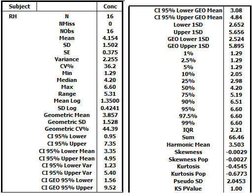
The NCA object creates seven results worksheets: Dosing Used, Exclusions, Final Parameters, Final Parameters Pivoted, Partial Areas, Plot Titles, Slopes Settings, and Summary Table. Selections from the Final Parameters and Summary Table worksheets are shown below.
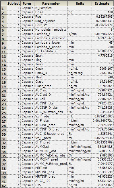
Final Parameters worksheet
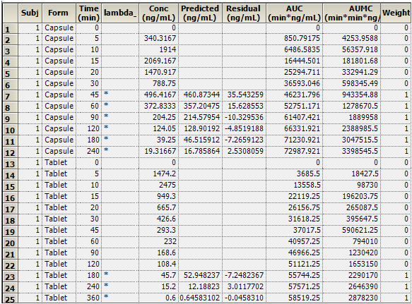
Summary Table worksheet
Plots
A total of 12 plots are generated; one for each of two formulations, for each of the six subjects. The first two charts for subject one are shown below.
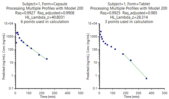
Plots for subject one, capsule and tablet formulation
Confirm pharmacokinetic modeling functions
-
Select File > Load Project. The Load Project dialog is displayed.
-
Navigate to <Phoenix_install_dir>\application\Examples\WinNonlin.
-
Select PK_Model.phxproj and click Open.
This project contains: -
Expand the workflow node.
-
Select the PK Model object in the Object Browser.
-
Select items in the Setup tab list to explore the model’s data mappings and option settings.
The imported PK Model object uses PK Model 3, which is a one-compartment model with 1st order absorption. -
Execute the object.
•A dataset worksheet (study1).
•An XY Plot object.
•A PK model object.
The PK Model object’s output worksheets partially include Condition Numbers, Diagnostics, Dosing Used, Final Parameters, Initial Estimates, Secondary Parameters, and Summary Table. The Final Parameters, Secondary Parameters, and Summary Table worksheets are shown below.
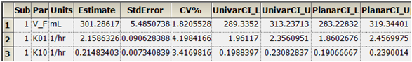
Final Parameters worksheet
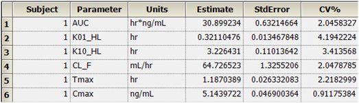
Secondary Parameters worksheet
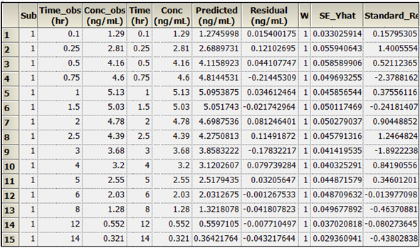
Summary Table worksheet
The Core output text results include all model settings and iterations, including the output from the worksheets. Any model errors would be listed here. Part of this file is shown below.
…
Listing of input commands
MODEL 3
NVAR 3
NPOI 1000
XNUM 2
YNUM 3
NCON 3
CONS 1,2,0
METH 2‘Gauss-Newton (Levenberg and Hartley)
ITER 50
INIT 0.25,1.81,0.23
MISS ‘.’
DATA ‘WINNLIN.DAT’
BEGIN
The Settings file lists all the settings used to specify the noncompartmental analysis. Part of this file is shown below.
…
Main: PK Model.Data.study1
Sort: Subject
Time: Time [hr]
Concentration: Conc [ng/mL]
Carry:
Dosing: (Internal)
Initial Estimates: (Internal)
Units: (Internal)
***** Other Parameters *****
…
PK 3-[PK]
Gauss-Newton (Levenberg and Hartley)
Convergence criteria of 0.0001 used during minimization process
50 maximum iterations allowed during minimization process
The plot results include Observed Y and Predicted Y vs X, Partial Derivatives Plot, Predicted Y vs Observed Y, Predicted Y vs X, Residual Y vs Predicted Y, and Residual Y vs X. Some plot results are shown below.
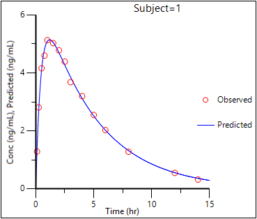
Observed Y and Predicted Y vs X
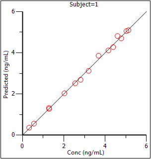
Predicted Y vs Observed Y
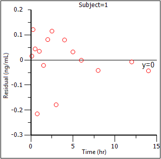
Residual Y vs X
Confirm bioequivalence functions
-
Select the Install Test project in the Object Browser.
-
Select File > Import.
-
In the Import File(s) dialog, navigate to <Phoenix_install_dir>\application\Examples\WinNonlin\Supporting files.
-
Select the file Seq2Per4.csv and click Open.
-
In the File Import Wizard dialog, click Finish. The dataset is added to the project Data folder.
-
Select the project workflow in the Object Browser and then select Insert > Computation Tools > Bioequivalence.
The Bioequivalence object is added to the workflow in the Object Browser. -
Use the pointer to drag the Seq2Per4 worksheet from the Data folder to the Main Mappings panel.
The Seq2Per4 dataset is mapped to the Bioequivalence object. -
Use the option button in the Main Mappings panel to map AUC to the Dependent context.
The following data types are automatically mapped to contexts when the dataset is mapped to the Bioequivalence model.
Sequence is mapped to the Sequence context.
Subject is mapped to the Subject context.
Period is mapped to the Period context.
Formulation is mapped to the Formulation context.
AUC is mapped to the Dependent context. -
In the Model tab (located below the Setup tab), ensure that Crossover is selected as the Type of study, Average is selected as the Type of Bioequivalence, and R is selected as the Reference Formulation.
-
Select the Fixed Effects tab, which is located below the Setup tab.
Ln(x) is automatically selected in the Dependent Variables Transformation menu. Do not change this setting. -
Execute the object.
Note:The default settings for a new Bioequivalence model are Crossover as the type of study and Average as the type of bioequivalence.
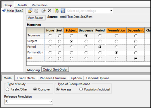
Settings for a Bioequivalence model
The bioequivalence model worksheet output partially includes Average Bioequivalence, Diagnostics, Final Fixed Parameters, Final and Initial Variance Parameters, Least Squares Means, and Sequential Tests. The Diagnostics, Final Variance Parameters, and Sequential Tests worksheets are shown below.
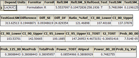
Average Bioequivalence worksheet
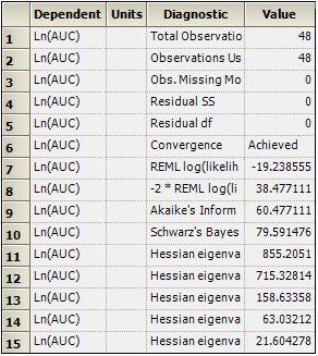
Diagnostics worksheet
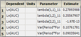
Final Variance Parameters worksheet
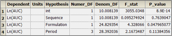
Sequential Tests worksheet
This concludes the Phoenix installation tests.
Test installation of Phoenix NLME
This section tests Phoenix WinNonlin’s population modeling functions. This test is not intended as a full validation of population modeling.
Users who have purchased a license for Phoenix NLME can use the Maximum Likelihood Models object to create and test population models. After Phoenix is installed, follow the steps below to confirm that population modeling is working correctly.
If any problems are encountered during this installation test, report the issue to Customer Support.
Start Phoenix and create a project
-
Double-click the Phoenix icon (
 ) on your desktop to start Phoenix.
 -
Select File > New Project to create a new project. A new project is created in the Object Browser.
-
Name the new project Installation Project.
-
To verify active licenses select Help > About Phoenix. For this installation test to work users must have an active license for Phoenix NLME 8.1.
Confirm population modeling functionality
This example verifies that the Phoenix NLME license and the Minimal GNU C++ compiler are correctly installed and configured. If Phoenix is being used without population modeling functionality, then skip this part of the installation test.
-
Select File > Import.
-
In the Import File(s) dialog, navigate to <Phoenix_install_dir>\application\Examples\NLME\Supporting files.
-
Select theopp.csv and click Open.
-
In the File Import Wizard dialog, click Finish. The dataset is added to the project Data folder and the worksheet is opened.
-
Select the workflow object in the Object Browser.
-
Select File > Load Workflow Template.
-
In the dialog, navigate to <Phoenix_install_dir>\application\Examples\NLME\Supporting files.
-
Select Diagonal Model.phxtmplt and click Open.
WinNonlin template files store information about settings and internal worksheets, but do not store external data sources.
The template file adds a one-compartment, 1st order absorption model that uses weight as a covariate. The model uses the FOCE L-B (First Order Conditional Estimation with the Lindstrom-Bates iterative algorithm) run method. -
Select the Structural, Parameters, and Run Options tabs to examine the model configuration.
The Parameters tab contains several sub-tabs that list fixed effects, random effects, and covariates. -
Use the pointer to drag the theopp worksheet from the Data folder to the Main Mappings panel.
The theopp dataset is mapped to the Diagonal model and the study variables xid, dose, time, yobs, and wt are automatically mapped to the contexts ID, Aa, Time, CObs, and wt, respectively. -
Execute the object.
-
Close the NLME Job Status dialog by clicking the X in the upper right corner.
Verify the results
-
Select the Verification tab.
The Verification Results state that the model successfully executed, and that no errors occurred. -
Select the Results tab.
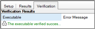
Verification tab
The model object produces text files, plots, and worksheets. The output types are listed below.
The model creates 23 worksheet results. Some of the output worksheets are Eta, EtaCovariate, Omega, and Theta. Not all worksheets listed under Output Data contain results.
Confirm the accuracy of some of the output in order to complete the installation test.
-
In the Output Data, select the Theta worksheet and confirm that the following estimates are the same (after rounding):
tvKa 1.55696
tvV 0.455554
tvCl 0.0402882
stdev0 0.692202
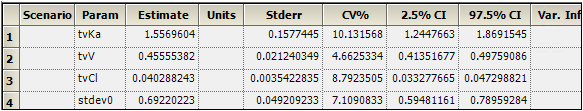
Theta worksheet
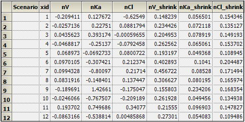
Eta worksheet
Thirty-nine plots are listed in the Plots section. Not all listed plots have results.
-
In the Plot output, select Pop CWRES vs PRED and compare it to the screen shot below:
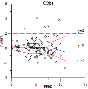
Pop CWRES vs PRED
The Maximum Likelihood Models object creates six text files. The Settings text file lists model settings, part of which is shown below.
…
Sort:
ID: xid
Aa: dose
Time: time
CObs: yobs
wt: wt
…
test(){
deriv(Aa = -Ka * Aa)
deriv(A1 = Ka * Aa - Cl * C)
dosepoint(Aa)
C=A1/V
error(CEps = 1)
observe(CObs = C + CEps)
stparm(Ka = tvKa * exp(nKa))
stparm(V = tvV * exp(nV))
stparm(Cl = tvCl * exp(nCl))
covariate(wt)
fixef(tvKa = c(, 1.54697,))
fixef(tvV = c(, 0.455465,))
fixef(tvCl = c(, 0.0402979,))
ranef(diag(nV, nKa, nCl)=c(0.01809, 0.41265, 0.06997))
}
------------------------------------
id("xid")
time("time")
dose(Aa<-"dose")
covr(wt<-"wt")
obs(CObs<-"yobs")
table(file=”posthoc.csv”, time(0), Ka,V,Cl)
------------------------------------
Run Options
Method: FOCE L-B
N Iter:1000
Input sorted by subject+time
Enabling automatic log transform (if applicable)
ODE solver method: matrix exponent
Method of computing standard errors: Central Diff
Hessian standard errors
Confidence Level %95
Simple run was performed
This concludes the installation test for Phoenix NLME. Close project without saving it.
