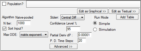
The Run Options tab allows users to determine how Phoenix executes a model. For individual modeling, the jobs are always run locally using the run method Naive-pooled, which cannot be changed. Population modelers have many more run options.
Individual modeling run options
Population modeling run options
For detailed explanations of Maximum Likelihood Models run methods, see “Run modes”.
Individual modeling run options
The following options are displayed on the Run Options tab when the Population? checkbox is unchecked.

-
In the N Iter field, type the maximum number of iterations to use with each modeling run (the default is 1000 and the maximum is 10,000).
-
Check the Sort Input? checkbox (the default) to sort the input by subject and time values.
When checked, the data is automatically sorted by ID (up to 5 levels of ID) and then by Time (if the model is time-based). Unchecking this option will process the data in the order given in the input dataset, and thus if the same subject ID is present in the dataset but the records are not consecutive they will be treated as two different subjects.
If a single ID entry within a column is non-numeric then the entire column is considered non-numeric, otherwise it is considered numeric. Note that non-numeric and numeric ID variables are sorted differently. For example, in numeric ID sorting, 2 comes before 10 but in non-numeric order 10 comes before 2.
If dosing information comes from a dosing worksheet (external or internal) then Sort Input? is automatically selected because of the need to merge the dosing and main worksheets. Similarly, if the model has a parameter worksheet that provides initial values, the Sort Input? option is automatically selected because it requires merging and thus sorting over sub-populations or individuals.
The Sort Input? option is available for population modeling as well. -
In the Max ODE menu, select one of the ODE (ordinary differential equations) solver methods: matrix exponent, auto-detect, non-stiff DVERK, stiff, non-stiff DOPRI5.
For more on ODE methodology, see “Differential equations in NLME”.
Standard errors for the parameter estimators for individual models are computed using the Hessian method. The Hessian method evaluates the uncertainty matrix as R-1, where R-1 is the inverse of the second derivative matrix of the -2*Log Likelihood function.
Note:Computing the standard errors for a model can be done as a separate step after model fitting. This allows the user to review the results of the model fitting before spending the time computing standard errors.
For engines other than QRPEM:
– After doing a model fitting, accept all of the final estimates of the fitting.
– Set the number of iterations to zero.
– Rerun with a method selected for the Stderr option.
For QRPEM, use the same steps, but also request around 15 burn-in iterations.
-
In the Stderr menu, select the method used to compute standard errors.
none (no standard error calculations are performed)
Central Diff for the second-order derivative of f uses the form:

Forward Diff for the second-order derivative of f uses the form:

The Stderr option is available for population modeling as well.
-
In the Confidence Level % field, enter the confidence interval percentage.
-
In the Partial Deriv dP field, enter the amount of perturbation to apply to parameters to obtain partial derivatives.
-
Enter the number of time steps in the P. D. Time Steps field.
Plots of the partial derivatives are spaced at this number of time vales over the whole time line. To get a coarse plot, specify a low number. To get a smoother plot, specify a larger number of steps.
