NonParametric Superposition

In pharmacokinetics it is often desirable to predict the drug concentration in blood or plasma after multiple doses, based on concentration data from a single dose. This can be done by fitting the data to a compartmental model with some assumptions about the absorption rate of the drug. An alternative method is based on the principle of superposition, which does not assume any pharmacokinetic (PK) model.

Phoenix’s nonparametric superposition object is used to predict drug concentrations after multiple dosing at steady state, and is based on noncompartmental results describing single dose data. The predictions are based upon an accumulation ratio computed from the terminal slope (Lambda Z). The feature allows predictions from simple (the same dose given in a constant interval) or complicated dosing schedules. The results can be used to help design experiments or to predict outcomes of clinical trials when used in conjunction with the semicompartmental modeling function.

Use one of the following to add the Nonparametric Superposition object to a Workflow:

Right-click menu for a Workflow object: New > NCA and Toolbox > Nonparametric Superposition.
Main menu: Insert > NCA and Toolbox > Nonparametric Superposition.
Right-click menu for a worksheet: Send To > NCA and Toolbox > Nonparametric Superposition.

Note:To view the object in its own window, select it in the Object Browser and double-click it or press ENTER. All instructions for setting up and execution are the same whether the object is viewed in its own window or in Phoenix view.

User interface description
Results
NonParametric Superposition methodology
NonParametric Superposition example

User interface description

Main Mappings panel
Administered Dose panel
Terminal Phase panel
Dosing panel
Options tab
Plots tab

Main Mappings panel

Use the Main Mappings panel to identify how input variables are used in the NonParametric object. NonParametric superposition requires a dataset containing time and concentration data, and sort variables to identify individual profiles. Required input is highlighted orange in the interface.

•None: Data types mapped to this context are not included in any analysis or output.

•Sort: Categorical variable(s) identifying individual data profiles, such as subject ID in a nonparametric analysis. A separate analysis is performed for each unique combination of sort variables.

•Time: The relative or nominal sampling times used in a study.

•Concentration: The measured amount of a drug in blood plasma.

Administered Dose panel

Using the Administered Dose panel is optional. When this panel is not used, it is assumed that the administered dose, or the dose associated with the data, is the same as the Loading Dose specified in the Regular Dosing tab, or the same as the dose at time zero specified in the Variable Dosing tab. Required input is highlighted orange in the interface.

Note:The sort variables in the dosing data worksheet must match the sort variables used in the main input dataset.

•None: Data types mapped to this context are not included in any analysis or output.

•Sort: Categorical variable(s) identifying individual data profiles, such as subject ID in a nonparametric analysis. A separate analysis is performed for each unique combination of sort variables.

•Administered Dose: The amount of drug given.

Terminal Phase panel

A dataset containing terminal phase information is options. If the dataset is available, use the Terminal Phase panel for mapping the start and end times for the terminal elimination phase for each profile. Use an internal worksheet to set the range (NPS does not use an extern worksheet mapping for Lambda Z setup.)

Note:The sort variables in the dosing data worksheet must match the sort variables used in the main input dataset.

•None: Data types mapped to this context are not included in any analysis or output.

•Sort: Categorical variable(s) identifying individual data profiles, such as subject ID in a nonparametric analysis. A separate analysis is performed for each unique combination of sort variables.

•Start and End: Start and end times for the terminal elimination phase. These contexts are generally not required. However, if the user maps an external worksheet to Terminal Phase, then the Start and End columns are required.

Dosing panel

The Dosing panel is only available if Variable is selected in the Dosing type menu. If the main input dataset used with the nonparametric superposition object contains variable times between doses, then use the Dosing panel to enter the separate time and dose values. Required input is highlighted orange in the interface.

•None: Data types mapped to this context are not included in any analysis or output.

•Time: Time that the drug is administered.

•Dose: The amount of drug administered.

Options tab

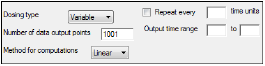
The Options tab allows users to select the dosing type, specify options related to regular and variable dosing, and enter dosing values for regular dosing.

In the Dosing Type menu, select the dosing interval type.

•Regular: For dosing at a regular time interval.

•Variable: For dosing at variable time intervals.

If variable dosing is selected then the Dosing panel is displayed in the Setup tab list. The Dosing panel is used to enter separate doses and times.

Selecting different dosing type changes the options in the Options tab. For regular dosing type options see “Regular dosing options”. For variable dosing type options see “Variable dosing options”.

In the Number of data output points field, type the number of data output points.
The default number of data points for regular dosing is 101. The default number of data points for variable dosing is 1001.
In the Method for computations menu, select the method used for interpolation and extrapolation of untransformed data.

•Linear: Uses only Linear interpolation. Use when data after Tmax is not necessarily exponentially declining.

•Log: For each dosing interval, uses Linear interpolation through the Tmax of that interval, and Log interpolation after Tmax.

Regular dosing options

In the Loading Dose field, type the initial dose used to calculate the AUC (area under the curve).
In the Maintenance dose field, type the maintenance dose used to calculate the AUC.
In the Tau field, type the dosing interval value.

Note:The value entered in the Tau field must match the time values used in the dataset. For example, if the time in the dataset is measured in hours and a dose is given once every day, type 24 in the Tau field.

Select the Display at steady state option button to have Phoenix generate the Predictions vs Time plot at steady state.
Select the Display N^th dose option button to have Phoenix generate the Predictions vs Time at a particular dose.
In the Display N^th dose field, type the dose used to generate the Predictions vs Time plot.

Variable dosing options

Select the Repeat every N time units checkbox to specify a repeating dosing regimen.
In the Repeat every N time units field, type the repeat time for one dosing cycle.

Note:The time units entered in the Repeat every N time units field must match the time units used in the Dosing panel. For example, if the dosing cycle repeats every 24 hours, type 24 in the Repeat every N time units field.

In the Output time range fields, type the start and end times used to create the predicted output data.

Plots tab

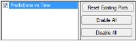
The Plots tab allows users to select whether or not plots are included in the output.

Use the checkboxes to toggle the creation of graphs.
Click Reset Existing Plots to clear all existing plot output.

Each plot in the Results tab is a single plot object. Every time a model is executed, each object remains the same, but the values used to create the plot are updated. This way, any styles that are applied to the plots are retained no matter how many time the model is executed.

Clicking Reset Existing Plots removes the plot objects from the Results tab, which clears any custom changes made to the plot display.
Use the Enable All and Disable All buttons to check or clear all checkboxes for all plots in the list. These buttons are most useful when there are many plots listed.

Results

NonParametric superposition generates worksheets containing predicted concentrations and Lambda Z values, as well as plots of predicted concentration over time for each sort level, and a summary plot.

•The Concentrations worksheet contains times and predicted concentrations for each level of the sort variables. If a regular dosing schedule is selected, this output represents times and concentrations between two doses at steady state. If a variable dosing schedule is selected, the output includes the times and concentrations within the supplied output range.

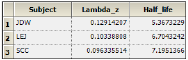
•The Lambda Z worksheet contains the Lambda Z value and the half-life for each sort key.

Note:NPS and NCA Best-Fit Lambda Z calculations can generate slightly different Lambda Z values (at the sixth significant digit) when the input data contains eight significant digits or more.

NPS stops if the last three points fail to compute Lambda Z (such as the last three points going uphill). If this situation occurs, you can execute NCA on the data using the default settings, and then map the NCA Slopes result to the Terminal Phase setup in the NPS object. The NCA execution will check further back in the dataset to see if a larger group of points ending with the last point will yield a valid Lambda Z.

NonParametric Superposition methodology

NonParametric superposition assumes that each dose of a drug acts independently of every other dose; that the rate and extent of absorption and average systemic clearance are the same for each dosing interval; and that linear pharmacokinetics apply, so that a change in dose during the multiple dosing regimen can be accommodated.

In order to predict the drug concentration resulting from multiple doses, one must have a complete characterization of the concentration-time profile after a single dose. That is, it is necessary to know C(t_i) at sufficient time points t_i, (i=1,2,…,n), to characterize the drug absorption and elimination process. Two assumptions about the data are required: independence of each dose effect, and linearity of the underlying pharmacokinetics. The former assumes that the effect of each dose can be separated from the effects of other doses. The latter, linear pharmacokinetics, assumes that changes in drug concentration will vary linearly with dose amount.

The required input data are the time, dosing, and drug concentration. The drug concentration at any particular time during multiple dosing is then predicted by simply adding the concentration values as shown in the next section (“Computation method”).

Note:User-defined terminal phases apply to all sort keys. In addition, dosing schedules and doses are the same for all sort keys.

Computation method

Given the concentration data points C(t_i) at times t_i, (i=1,2,…,n), after a single dose D, one may obtain the concentration C(t) at any time t through interpolation if t₁< t <t_n, or extrapolation if t > t_n. The extrapolation assumes a log-linear elimination process; that is, the terminal phase in the plot of log(C(t)) versus t is approximately a straight line. If the absolute value of that line’s slope is _z and the intercept is ln(), then C(t)= exp(–_zt) for t > t_n.

The slope _z and the intercept are estimated by least squares from the terminal phase; the time range included in the terminal phase may be specified by the user or, if not specified, estimates from the best linear fit (based on adjusted R² as in the Best Fit method in Noncompartmental Analysis) will be used. The half life is ln(2)/_z.

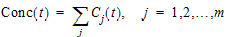
Suppose there are m additional doses D_j, j = 1,…,m, and each dose is administered after t_j time units from the first dose. The concentration due to dose D_j will be:

C_j(t)=(D_j / D)*C(t – t_j)

(1)

where t is time since the first dose and C(t – t_j) = 0 for t £ t_j.

The total predicted concentration at time t will be:

(2)

If the same dose is given at constant dosing intervals t, and t is sufficiently large that drug concentrations reflect the post-absorptive and post-distributive phase of the concentration-time profile, then steady state can be reached after sufficient time intervals. Let the concentration of the first dose be C₁(t) for 0 < t < t, so t is greater than t_n. Then the concentration at time t after n^thdose (i.e., t is relative to dose time) will be:

C_n(t) = C₁(t) + exp[–(t+t)] + exp[–(t+2t)]
+…+ exp[–(t+(n – 1)t)]

= C₁(t) + exp[–(t+t)]{1 – exp[–(n – 1)t]} / [1 – exp(–t)]

(3)

As , the steady state (ss) is reached:

C_ss(t)=C₁(t)+ exp[–(t+t)]/[1 – exp(–t)]

(4)

To display the concentration curve at steady state, Phoenix assumes steady state is at ten times the half life.

For interpolation, Phoenix offers two methods: linear interpolation and log-interpolation. Linear interpolation is appropriate for log-transformed concentration data and is calculated by:

C(t)=C(t_{i – 1})+[C(t_i) – C(t_{i – 1})]*[t – t_{i – 1}]/[t_i – t_{i – 1}],
t_{i – 1} < t < t_i

(5)

Log-interpolation is appropriate for original concentration data, and is evaluated by:

C(t)=exp{log(C(t_{i – 1}))+[log(C(t_i)) – log(C(t_{i – 1}))]*(t – t_{i – 1})/(t_i – t_{i – 1})}, t_{i – 1} < t < t_i

(6)

For additional information see Appendix E of Gibaldi and Perrier (1982). Pharmacokinetics, 2nd ed. Marcel Dekker, New York.

NonParametric Superposition example

This section uses the NonParametric Superposition object to predict plasma concentrations and effect-site concentrations at steady-state based on single-dose data. This feature allows for predictions on data that are otherwise difficult to model.

This example uses the output from the semicompartmental modeling example, detailed under “Semicompartmental model example”.

Knowledge of how to do basic tasks using the Phoenix interface, such as creating a project and importing data, is assumed.

SCM_NPS.phxproj) is available for reference in …\Examples\WinNonlin.

Set up an estimation of steady-state plasma concentrations

From within the SCM_NPS project created in the previous example, right-click Workflow in the Object Browser and select New > NCA and Toolbox > NonParametric Superposition.
Map the Semicompartmental Results worksheet as the input source for the NonParametric Superposition object:
Map Subject to the Sort context.
Leave Time mapped to the Time context.
Map Conc to the Concentration context.
Leave Ce mapped to None.
Leave Effect mapped to None.
In the Options tab below the Setup panel, type 50 in the Loading Dose field.
In the Maintenance Dose field type 50.
In the Tau (dosing interval) field type 4.

Execute and view the plasma estimation results

Click to execute the object. The results are displayed on the Results tab.

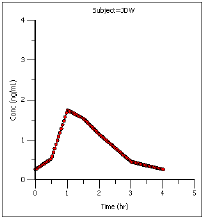
The NonParametric worksheet results provide predicted steady-state plasma concentrations and Lambda Z and half-life estimates.

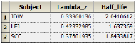
The plot output shows predicted steady state concentrations over time for each subject. The first subject’s plot is shown below.

Set up an estimation of steady-state effect-site concentrations

Select the NonParametric object’s Setup panel.
In the Main Mappings panel, re-map the data types to the following contexts:
Leave Subject mapped to the Sort context.
Leave Time mapped to the Time context.
Map Conc to None.
Map Ce to the Concentration context.
Leave Effect mapped to None.
Select Terminal Phase from the Setup list.
Check the Use Internal Worksheet checkbox.
For each row:
In the Start column, type 4.
In the End column, type 8.

Execute and view the effect-site concentration estimation results

Click to execute the object. The results are displayed on the Results tab.

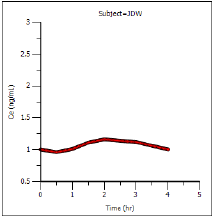
The new NonParametric worksheet results provide predicted effect site concentrations at steady-state and Lambda Z and half-life estimates.

The plot output shows predicted effect site concentrations at steady-state over time for each subject. The first subject’s graph is shown below.

Compute the steady-state effect

Now it is possible to compute the steady-state effect from the predicted steady-state concentrations at the effect site.

Select the PD Model object in the Object Browser.

The sample graph for PD model 103 is displayed in the Model Selection tab below the Setup panel. Note the effect formula for model 103 is E=E0*(1 – (C/(C+IC50))).

Select the NonParametric object in the Object Browser.
In the Results tab, right-click the Concentrations (effect site concentrations) worksheet and select Copy to Data Folder.

The worksheet is added to the project’s Data folder and renamed Concentrations from NonParametric.
In the Object Browser, select Concentrations from NonParametric in the Data folder.
In the Columns tab below the table, click Add under the Columns list.
In the New Column Properties dialog, the Numeric option button is selected by default. Do not change this setting.
In the Column Name field type Effect and click OK.

The Effect column is added in the Columns list and in the table in the Grid tab.
Use the Down Arrow button beside the Columns list to move the Effect column header to the bottom of the Columns list.
In the Object Browser, right-click Concentrations from NonParametric and select Edit in Excel.

Phoenix displays a message warning users that changes made in Excel are not recorded in Phoenix.
Click OK.

The worksheet is opened in Excel. If you see a pop-up dialog stating that the format and extension of the file do not match, click Yes to continue as the file is safe to open.

In Excel, enter the PD model 103 effect formula in the Effect column for each subject at time zero. Use the E0 and IC50 values from the PD Model object’s Final Parameters worksheet.
Select the cell in the Effect column at time zero for the first subject, JDW.
Type the effect formula shown below in the Effect column cell at time 0 (zero) for subject JDW, which is row 3.
= 102.93*(1-(C3/(C3+0.09))) (for subject JDW)
Repeat for the second and third subjects, LEJ (row 103) and SCC (row 203).
= 100.17*(1-(C103/(C103+0.09))) (for subject LEJ)
= 100.45*(1-(C203/(C203+0.08))) (for subject SCC)
After the Effect value formula is set up at time zero for each subject copy the formula to the other time points for each subject.

Because of the way Phoenix handles its interactions with Excel, users cannot use the Save As option in Excel to save the worksheet with a different name or to a different location. The Save option must be used.
Select File > Save.
Close Excel. Be sure to save the worksheet before closing Excel, or all changes are lost.
An Apply Changes message dialog is displayed.
Click Yes to apply the changes. An entry is written in the worksheet History tab noting that it was edited in Excel.
When asked whether to save formulas, select No so that the worksheet is editable in Phoenix.

The Concentrations from NonParametric worksheet now has Effect values derived from the equations used in the Excel edit and can still be used with operational objects.

Plot time vs effect

Once the steady-state effects and concentrations are generated it is possible to use the modified concentrations from NonParametric worksheet to plot time vs. effect for each subject by mapping the worksheet to an XY Plot object.

Right-click Workflow in the Object Browser and select New > Plotting > XY Plot.
Drag Concentrations from NonParametric from the Data folder to the XY Data Mappings panel:
Map Subject to the Group context.
Map Time to the X context.
Leave Ce mapped to None.
Map Effect to Y context.
Click to execute the object.

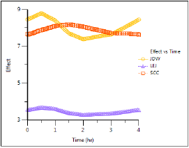
This concludes the Nonparametric superposition example.