Semicompartmental modeling was proposed by Kowalski and Karim (1995) for modeling the temporal aspects of the pharmacokinetic-pharmacodynamic relationship of drugs. Their model was based on the effect-site link model of Sheiner, Stanski, Vozeh, Miller and Ham (1979) to estimate effect-site concentration Ce, but uses a piecewise linear model for plasma concentration Cp rather than specifying a PK model for Cp. The potential advantage of this approach is reducing the effect of model misspecification for Cp when the underlying PK model is unknown.
Use one of the following to add a Semicompartmental Modeling object to a Workflow:
Right-click menu for a Workflow object: New > NCA and Toolbox > Semicompartmental Modeling.
Main menu: Insert > NCA and Toolbox > Semicompartmental Modeling.
Right-click menu for a worksheet: Send To > NCA and Toolbox > Semicompartmental Modeling.
Note:To view the object in its own window, select it in the Object Browser and double-click it or press ENTER. All instructions for setting up and execution are the same whether the object is viewed in its own window or in Phoenix view.
Use the Main Mappings panel to identify how input variables are used in the Semicompartmental object. Semicompartmental modeling requires a dataset containing time and concentration data, and sort variables to identify individual profiles. Required input is highlighted orange in the interface.
•None: Data types mapped to this context are not included in any analysis or output.
•Sort: Categorical variable(s) identifying individual data profiles, such as subject ID in a semicompartmental analysis. A separate analysis is performed for each unique combination of sort variables.
•Time: The relative or nominal dosing times used in a study.
•Concentration: The measured amount of a drug in blood plasma.
•Effect: The measured effect data.
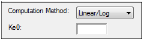
The Options tab allow users to select the computation method and the Ke0 value.
-
In the Computation Method menu, select the method Phoenix uses to perform the semicompartmental analysis.
•Linear uses a linear piecewise PK model.
•Log uses a log-linear piecewise PK model.
•Linear/Log start with linear to Tmax and then log-linear after Tmax; this is also the default option.
-
In the Ke0 field, type the value for the equilibrium rate constant.
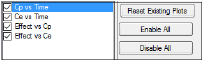
The Plots tab allows users to select whether or not plots are included in the output.
-
Use the checkboxes to toggle the creation of graphs.
-
Click Reset Existing Plots to clear all existing plot output.
Each plot in the Results tab is a single plot object. Every time a model is executed, each object remains the same, but the values used to create the plot are updated. This way, any styles that are applied to the plots are retained no matter how many time the model is executed.
Clicking Reset Existing Plots removes the plot objects from the Results tab, which clears any custom changes made to the plot display. -
Use the Enable All and Disable All buttons to check or clear all checkboxes for all plots in the list. These buttons are most useful when there are many plots listed.
The Semicompartmental model object generates four charts, one worksheet, and one text file.
Up to four plots are created for each profile. Each profile’s plot is displayed on its own page in the Results tab.
•Select each plot in the Results tab. Click the page tabs at the bottom of each plot panel to view the plots for individual profiles.
•If drug effect data is included in the dataset, Effect vs Ce and Effect vs Cp plots are also created.
|
Plot |
Content |
|
Ce vs Time |
Estimated effect site concentration vs. time. |
|
Cp vs Time |
Plasma concentration vs. time. |
|
Effect vs Ce |
Drug effect vs. the estimated effect site concentration. |
|
Effect vs Cp |
Drug effect vs. plasma concentration. |
A text file called Settings is also created. It lists the user-specified settings in the Semicompartmental object
The Semicompartmental object creates a worksheet called Results. The Results worksheet contains the following data:
•Sort variables, if any are used
•Time points used in the study
•Drug concentration levels in blood plasma
•Ce, the estimated effect site concentration
•Effect data, if included
•Any units associated with the time and concentration columns in the input data are carried through to the semicompartmental modeling output
Semicompartmental calculations
Ke0. This function should be used when a counterclockwise hysteresis is observed in the graph of effect versus plasma concentrations. The hysteresis loop collapses with the graph of effect versus effect-site concentrations.
A scientist developing a PK/PD link model based upon simple IV bolus data can use this function to compute effect site concentrations from observed plasma concentrations following more complicated administration regimen without first modeling the data, i.e., semicompartmental modeling determines if the hysteresis can be collapsed using an effect compartment, without requiring a full compartmental model. The results can then be compared to the original datasets to determine if the model suitably describes pharmacodynamic action after the more complicated regimen.
Drug concentration in plasma Cp for each subject is measured at multiple time points after the drug is administrated. To minimize the bias in estimating Ce, the time points need to be adequately sampled such that accurate estimation of the AUC by noncompartmental methods can be obtained. Effect-site link model is used and the value of the equilibration rate constant ke0 that accounts for the lag between the Cp and the Ce curves is required. The default option is for a piecewise Linear/Log model to be assumed for Cp.
In the effect-site link model proposed by Sheiner, Stanski, Vozeh, Miller and Ham (1979), a hypothetical effect compartment was proposed to model the time lag between the PK and PD responses. The effect site concentration Ce is related to Cp by first-order disposition kinetics and can be obtained by solving the differential equation:
|
|
(1) |
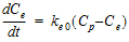
where ke0 is a known constant. In order to solve this equation, one needs to know Cp as a function of time, which is usually given by compartmental PK models.
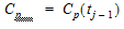
Here, use a piecewise linear model for Cp:
|
|
(2) |

where:
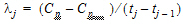
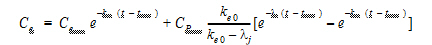
Using the above two equations can lead to a recursive equation for Ce:
|
|
(3) |

The initial condition is Cp(0)=Ce(0) =0.
One can also assume a log-linear piecewise PK model for Cp:
|
|
(4) |

where, 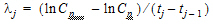 , and;
|
|
(5) |
 and
and  are estimated by a linear regression, assuming
 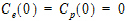 .
.
Phoenix provides three methods. The ‘linear’ method uses linear piecewise PK model; the ‘log’ method uses log-linear piecewise PK model; the default ‘log/linear’ method uses linear to Tmax and then log-linear after Tmax. The Effect field is not used for the calculation of Ce but when it is provided, the E vs Cp and E vs Ce plots will be plotted.
Kowalski ad Karim (1995). A semicompartmental modeling approach for pharmacodynamic data assessment, J Pharmacokinet Biopharm 23:307–22.
Sheiner, Stanski, Vozeh, Miller and Ham (1979). Simultaneous modeling of pharmacokinetics and pharmacodynamics: application to d-tubocurarine. Clin Pharm Ther 25:358–71.
Semicompartmental model example
The examples of semicompartmental modeling and nonparametric superposition use the dataset in the file PK.CSV, which is located in the Phoenix examples directory. The data are from an early Phase I PK/PD trial. Quick input is sought for the design of a seven day multiple dose study. However, the profiles are irregular, and it is not easy to apply a compartmental modeling approach to the data.
Knowledge of how to do basic tasks using the Phoenix interface, such as creating a project and importing data, is assumed.
SCM_NPS.phxproj) is available for reference in …\Examples\WinNonlin.
Explore the input data
-
Create a new project.
-
Rename the project as SCM_NPS.
-
Import the file …\Examples\WinNonlin\Supporting files\PK.CSV.
In the File Import Wizard dialog, select the Has units row option.
The braces in the Effect column header indicate that the units are nonstandard and will be carried throughout the analysis but they cannot be used in unit conversions. -
Right-click Workflow in the Object Browser and select New > Plotting > XY Plot.
-
Drag the PK worksheet from the Data folder to the XY Data Mappings panel.
Map Subject to the Group context.
Map Time to the X context.
Map Conc to the Y context.
Leave Effect mapped to None. -
Click
 to execute the object. The results are displayed on the Results tab.
The plot indicates that compartmental modeling might be problematic. The data are highly variable. -
Return to the Select panel and re-map the input data:
Leave Subject mapped to the Group context.
Map Time to None.
Map Conc to the X context.
Map Effect to the Y context.
The graph display options are located in the XY Plot's Options tab. -
In the Options tab below the Setup panel, select Graphs > Effect vs Conc in the menu tree.
-
Clear the Sort X Values checkbox.
Clearing the Sort X Values checkbox tells Phoenix to not sort the dataset by ascending concentration values before creating the XY plot. -
Click
 .
.
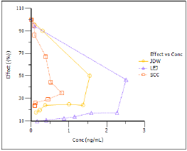
Notice the hysteresis in the plot. Semicompartmental modeling supports calculation of effect-site concentrations based on Ke0. In this example, pre-clinical studies indicated that the Ke0 is between 0.2 and 0.3 per hour in rats and dogs.
Set up the Semicompartmental object
This example estimates effect-site concentrations using semicompartmental modeling:
-
Right-click Workflow in the Object Browser and select New > NCA and Toolbox > Semicompartmental Modeling.
-
Drag the PK worksheet from the Data folder to the Main Mappings panel.
Map Subject to the Sort context.
Leave Time mapped to the Time context.
Map Conc to the Concentration context.
Leave Effect mapped to the Effect context. -
In the Options tab below the Setup panel, type 0.25 in the Ke0 field.
Execute and view the Semicompartmental results for the PK data
-
Click
 to execute the object. The results are displayed on the Results tab.
The Semicompartmental Model provides both workbook and graph output.
The Results worksheet shows the calculated concentration of the drug in the effect compartment, Ce, at each Time in the input dataset, along with the input Conc and Effect data, for each subject.
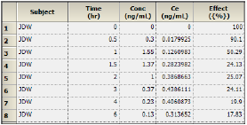
Part of the Semicompartmental Results worksheet
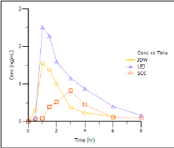
The Semicompartmental object generated four plots for each subject.
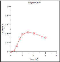
Effect-compartment concentration (Ce) over time (Ce vs Time)
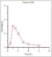
Concentration over time (Cp vs Time)
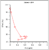
Effect as a function of Ce (Effect vs Ce)
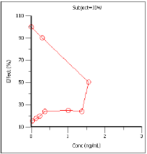
Effect over concentration (Effect vs Cp)
Based on the plots, PD model 103, an Inhibitory Effect E0 model, is appropriate to use to model the concentration in the effect compartment (Ce) versus effect relationship.
Model the pharmacodynamics
-
Right-click Workflow in the Object Browser and select New > WNL 5 Classic Modeling > PD Model.
-
Map the Semicompartmental Results worksheet as the input source for the PD Model object:
Map Subject to the Sort context.
Leave Time mapped to None.
Leave Conc mapped None.
Map Ce to the X variable context.
Map Effect to the Y variable context. -
In the Model Selection tab below the Setup panel, check the model Number 103 checkbox.
The default model parameter options are used. Phoenix generates initial parameter values and parameter bounds. To view the parameter option settings, select the Parameter Options tab.
Execute and view the PD Model results for the Semicompartmental output
-
Click
 to execute the object. The results are displayed on the Results tab.
Phoenix analyzes each subject separately and includes all time points per subject.
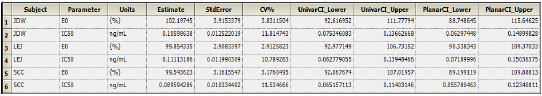
The Final Parameters output provides estimates for E0 and IC50 for each subject. These are used later to predict steady-state effect values. -
Click Observed Y and Predicted Y vs X under Plots.
The Observed Y and Predicted Y vs X plot illustrates the fit of PD model 103 to the effect data when Ce from Semicompartmental modeling is used as the measure of exposure. The Observed Y and Predicted Y vs X plot for the first subject is shown below.
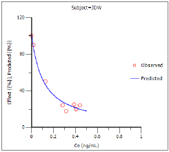
The other plots address model fit.
The NonParametric superposition example uses the output from this example. You may wish to save this project or leave the project open if you are continuing with the NonParametric superposition example.
