Note:The graphical model interface is a free-form model building interface. It is much more sophisticated than the built-in model, which means user error is more likely. It is recommended for advanced users.
To use the graphical editor to create the structural model:
•Click Edit as Graphical.
•In the displayed dialog, click Yes to confirm using the graphical editor.
•If Closed form? is currently checked, a second dialog is presented notifying the user that closed-form will not be used. This is because graphical models are built with differential equations. Click Yes to continue.
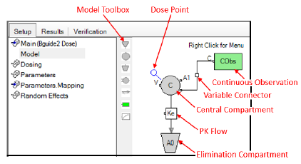
Example of a one-compartment, 1st order absorption PK model
When the graphical editor is in use, the Edit as Graphical button changes to Use Builtin. Click this button to return to the built-in model interface.
The Main Mappings, Dosing, Parameters, and Parameters.Mappings panels and all tabs except the Structure tab work the same in the Graphical model as they do in the built-in model. If no model elements are selected in the Model panel then the Structure tab displays the model parameters, statements, and scale control. Use the pointer to move the slider  right or left to adjust the graphical model scale, which makes the model picture larger or smaller. If a compartment is selected, then the compartment type and type-specific settings are displayed in the Structure tab.
Users can specify the model using the Model toolbox or the right-click menu. The right-click Insert menu allows users to insert compartments, flows, observations, PD blocks, structural parameters, and other model elements. Users can also cut, copy, paste, and manipulate model elements. (The difference between Replace and Insert is that the former replaces the selected objects in the diagram with the contents of the clipboard while trying to retain wire and flow connections. The latter just copies the contents of the clipboard into the diagram.)
|
Compartment |
Absorption ( |
|
|
|
Central ( |
|
|
|
Peripheral ( |
|
|
|
Elimination ( |
|
|
Flow ( |
|
|
|
Observation |
Continuous ( |
|
|
|
Categorical |
|
|
|
Event |
|
|
|
Count |
|
|
|
LL |
|
|
PD |
Emax ( |
|
|
|
Linear |
|
|
|
Indirect |
|
|
|
Effect Cpt |
|
|
Parameter |
|
|
|
Procedure |
|
|
|
Expression |
|
|
|
Annotation |
|
|
|
PBPK |
|
 )
) )
) )
) )
) )
) )
) )
)Caution:When switching from a PK/Emax, or PK/Indirect built-in to a Graphical model, verify the tab settings. In particular, the Freeze PK? checkbox, when checked in the built-in model, can become unchecked when switching to Graphical.
Absorption compartment options
This PK compartment is used as an input site for doses following a first-order input function. By default, flows connecting an absorption compartment to another compartment use a first-order function. That function can be changed by specifying PK flow options in the Structure tab. Connect an absorption compartment to another compartment via a PK flow to create a 1st-order absorption PK model.
-
Use the Model toolbox or select Insert > Compartment > Absorption from the right-click menu.
-
Absorption compartment work the same as the central compartment, (except there is no Conc option to add volume and concentration parameters). Refer to “Central compartment options” for details on setting these parameters.
Caution:Be careful not to use the same names for the volume and concentration parameters in different compartments.
-
Drag the dosing variable square from the absorption compartment to the central compartment dosing variable square.
Central compartments can be connected to other PK compartments, including at least one elimination compartment (unless no drug leaves the body), by using a PK flow. Any number of central and peripheral compartments can be connected together, with one exception: if a set of PK compartments using volume parameters are connected by PK flows parameterized in microconstants, there can be only one central compartment.
-
Use the Model toolbox or select Insert > Compartment > Central from the right-click menu.
-
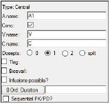
If desired, modify the default dosing variable name in the A name field.
Typically, A1 is used for intravenous input and Aa is used for extravascular input. -
Check the Conc checkbox (the default) if the compartment has concentration or volume parameters; uncheck it if there are no concentration or volume parameters.
The Conc checkbox controls the parameterization of the compartment. Selecting it adds the volume parameter V and the concentration parameter C to the model. When the checkbox is cleared, the compartment has no volume or concentration parameters, and can be useful for certain compartmental PD models. -
In the fields for the other structural parameters, enter names for each parameter.
-
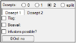
Select a Dosepts option button (0, 1, 2, or split) to specify the number of dose points used by the central compartment. Select split to split dosing into the central compartment between two dosepoints.
Dose points can be defined for any PK compartment. The time(s) and amount(s) of doses are defined in the dataset. Each drug can have multiple formulations. For example, a drug can have one formulation dosing into the central compartment (IV) and another formulation dosing into an absorption compartment (oral or intramuscular). A drug model can include any number of different formulations and different drugs.
Note:Option 2 requires the dosing data to be in separate columns in the input dataset. Option split requires the data to be in the same column.
If 1, 2, or split dose points are selected, users can add time delay parameters, bioavailability expressions, add infusions, and specify zero-order absorption options. For 2 or split, these parameters can be set for each dose point by selecting the Dosept 1 and Dosept 2 tabs.
-
Check the Tlag checkbox to add a time delay parameter to the model. Enter the time lag expression in the field.
-
Check the Bioavail checkbox to measure bioavailability in the central compartment. Enter the bioavailability expression in the field.
Bioavailability expressions can be entered as a numerical value or a parameter. For example, if a user enters 0.5, half the drug goes into the compartment.
To estimate bioavailability, a parameter must be used instead of a number. For example, a user can type F (fraction of dose absorbed parameter) in the Bioavail field to estimate drug availability. If new parameter names are used in the expression, these will have to be inserted into the model. See “Parameter block” for Parameter block usage instructions.
If users want to estimate bioavailability using multiple dosing routes, then a second parameter like 1-F can be entered in the Dosept 2 tab. Using multiple dosing routes and bioavailability parameters can be useful when modeling first- and second-pass absorption rates. -
Check the Infusions possible? checkbox if the dosing uses infusions.
•A dosing parameter rate, such as Aa Rate or A1 Rate, is added to the contexts in the Main Mappings panel.
•A Duration? checkbox is also added in the Structure tab. Checking this box causes the context A1 or Aa Rate to change to A1 or Aa Duration.
-
Click 0 Ord: No multiple times to toggle through the zero-order options:
•No: There is no zero-order input.
•Rate: The drug is introduced into the system at a constant rate. Enter the zero-order rate expression in the field, either as a parameter or a numeric value.
•Duration: The drug is introduced over a finite period of time, or duration. Enter the zero-order duration expression in the field, either as a parameter or a numeric value.
-
Select the Sequential PK/PD? checkbox if the PK model is part of a PK/PD model that is being fitted sequentially.This will freeze the PK portion of the model and turn its random effects into covariates. See “Sequential PK/PD Population Model Fitting” for more information.
Peripheral compartment options
Peripheral compartments can be connected to other PK compartments, including central and elimination compartments, by using a PK flow. If there is only one central compartment, the volumes of the peripheral compartments are determined by their surrounding constraints, or flow parameters.
-
Use the Model toolbox or select Insert > Compartment > Peripheral from the right-click menu.
-
Peripheral compartment options work the same as the central and absorption compartment options. Refer to “Central compartment options” for details on setting these parameters.
Elimination compartment options
The elimination compartment (which is shown as a urinecpt code statement) can be connected to any other PK compartment via a PK flow. The only difference between urinecpt and deriv is that urinecpt is ignored when determining a steady-state condition.
-
Use the Model toolbox or select Insert > Compartment > Elimination from the right-click menu.
-
Elimination compartment options work the same as the central compartment options, (except there is no Conc option to add volume and concentration parameters). Refer to “Central compartment options” for details on setting these parameters.
-
The fraction excreted (Fe) is an additional parameter that can be include in the code statement, as shown in the following example statement:
urinecpt(A0=(A1*Ke)
,fe=Fe
)
-
To indicate that the elimination compartment is set to zero right after being observed, edit the model as textual and change the PML code to:
observe(UrineObs=A0+eps, doafter={A0=0; })
Use a PK flow to represent a mass flow between PK compartments. To connect two PK compartments with a flow:
-
Click the flow button in the Model toolbox, or right-click and select Insert > Flow.
-
Use the pointer to click on the first and second PK compartments of the flow.
Note that lag time for an absorption model is indicated in the absorption or central compartments.
Different types of default PK flows are added depending on which compartments they connect:
•If the absorption compartment is connected to a central, peripheral, or elimination compartment, the default PK flow is a micro parameter, one-way flow. The default parameter name for the PK flow changes depending on the direction on which the flow moves, and on which compartments are being connected. For example, if the flow moves from the absorption compartment to another compartment, the parameter name for the forward movement (Kfwd) is Ka. The default parameter name for any backward PK flow is K12.
•The default PK flow between the central or peripheral compartments and the elimination compartment is named CL, and it is a clearance/volume parameter, one-way flow.
•The default PK flow between the central and peripheral compartments is named Q, and it is a clearance/volume parameter, with a two-way flow.
To specify PK flow options
-
Use the pointer to select a PK flow.
-
Click Parm multiple times to toggle through the parameterization options for the model.
•Micro: Enter a variable name for the flow into the second compartment in the Kfwd field or use the default. If the 2Way checkbox is also checked, enter a variable name for the flow back into the first compartment in the Kbak field.
•Clearance/Volume: Enter a variable name for the clearance in the CL field or use the default.
•Saturating: Enter variable names in the Vmax field for the maximum metabolic rate and in the Km field for the fractional metabolic rate or use the defaults.
-
Click the 2Way checkbox to change the PK flow to a two-way flow; uncheck it to create a one-way flow.
-
Click Draw multiple times to toggle through the options for drawing the PK flow in the Graphical model interface.
•Diagonal: Draws the diagonal flow.
•Horizontal First: Draws the flow horizontally from the first compartment.
•Vertical First: Draws the flow vertically from the first compartment.
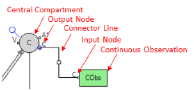
The Continuous Observation block links a model variable such as excreted amount, or plasma concentration, to observed data. The observations are normally distributed around the value of the model variable with some standard deviation prescribed by the error model. When estimating model parameters, the likelihood of an observation is obtained from the normal distribution. When simulating data, the observations are generated by sampling values from the standard normal distribution and applying them to the terms in the error model.
-
Insert a Continuous Observation block by using the Model toolbox or selecting Insert > Observation > Continuous from the right-click menu.
-
Place the pointer over an output node on a compartment or a block. The connector is surrounded by a blue circle when it is selected. The Continuous Observation block can be connected to any PK compartment, observation block, PD block, or parameter block.
-
Drag the output node connector to the C input node on the Continuous Observation block.
A line is displayed that represents the connection between the Continuous Observation block and the compartment or block.
To delete a connection
-
Select the square in the middle of the connector line. The line is surrounded by a blue square when it is highlighted.
-
Right-click the square and select Insert > Delete.
To specify continuous observation options
-
Use the pointer to select a Continuous Observation block.
-
In the Name field, enter a name for the Continuous Observation block or use the default name of CObs.
-
The rest of the options are the same as in the built-In model.
Use the Categorical Observation block to model multinomial data. The data should be given as integer (whole) number values, such as 0, 1, 2, etc. A key feature of the Categorical Observation block is the ability to use model variables to affect the probability of observing data in a particular category. For instance, the Categorical Observation block could be used to link the probability of a patient reporting adverse effects of a given type to the administered dose or even drug concentration.
The default settings for the Categorical Observation block give a 50% chance of a zero or one output when the input value is zero. The probability of a one output increases as the input value increases from zero.
-
Insert a Categorical Observation block by selecting Insert > Observation > Categorical.
The Categorical Observation block can be connected to any PK compartment, observation block, PD block, or parameter block. See the Continuous Observation block section for instructions on adding and deleting a connection.
To specify categorical observation options
-
Use the pointer to select a Categorical Observation block.
-
In the Mtn field, enter a name for the Categorical Observation block or use the default name.
-
Check the Inhibitory checkbox to set the output values to decrease as the input increases.
-
In the Link menu, select the inverse link function.
This function determines the shape of the demarcation between output values as a function of inputs. This is the inverse of the link function sometimes used in fitting data. In the equations listed below, i is the input variable value, o is the offset between a given set of outputs such as zero or one, and p is the probability of getting a specific output, given i and o.
Inverse link functions include:
•Logit: the inverse of the sigmoid function. p=ei+o/(1+ei+o)
•Probit: the inverse cumulative distribution function. p=G(i+o) where G is the cumulative normal distribution.
•Log-log: the logarithmic function. p=exp(–e–i+o)
•CLog-log: complementary logarithmic function. p=i+o (truncated to the interval [0,1])
-
In the Slope field, type the slope expression.
-
In the N outcomes menu, click (-) to decrease the number of outcomes, and click (+) to increase the number of outcomes.
N outcomes corresponds to the number of categorical output values. For example, if N outcomes is three, the output could equal zero, one, or two, depending on the input value. The minimum number of outcomes is two. -
In the Icept field, type the intercept expression.
Enter an expression representing the negative value of the input value that gives a 50% probability of outputting either of the adjacent output values. This is the negative of the offset between outputs. Because it is the negative, the values should be entered in descending numerical order. Use the syntax for expressions, described under “.“Syntax for text expressions and statements”
Each extra outcome that is added to the categorical observation adds an extra Icept field. The first Icept field is labeled Icept10. The second Icept field is labeled Icept21. Each extra Icept field is labeled Icept32, Icept43, Icept54, and so forth.
For more information on the use of the Categorical Observation block see “Multi statement for Multinomial models”.
Make sure the Model Text tab shows an entry for the observation in the Column Definition Text field. It is displayed as “obs([block name]<-[“column name”]). If there is no entry, type it in the User-Provided Extra Column Definition Text field.
An Event block represents an unscheduled event. Observations take the form of indicator variables for the event: 1 if the event occurs at the time of the observation, or 0 (zero) if the event has not yet occurred at the time of the observation.
The likelihood of the observation is determined by integrating the hazard over the length of the sampling interval, so that at the end of the interval the expected number of events are computed. The expected, or mean, number of events is made the mean of a Poisson distribution. A sample is taken at random from that Poisson distribution at each sampling interval to say how many, if any, events occurred.
The number of events during each sampling interval, which is only one if a probability is entered, is added to the N output variable of the event block.
An event block represents an unscheduled event. One record is created in the results for each evaluation period during which the event is triggered. Each record indicates the time, the censor value (one for event occurrence; zero for right-censored), and a sequence number showing the total number of events having occurred for a given subject.
Note:Censor values in the results are zero for censored events and one for non-censored event records, where the event happened.
-
Insert an Event Observation block by selecting Insert > Observation > Event from the right-click menu.
The Event Observation block can be connected to any PK compartment, observation block, PD block, or parameter block. See the Continuous Observation block section for instructions on adding and deleting a connection.
To specify event observation block options
-
Use the pointer to select an Event Observation block.
-
In the Evt field, enter a name for the Event Observation block or use the default.
-
Check the Has Input? checkbox if the slope term comes from elsewhere in the model and enter the hazard slope expression in the Slope field.
An input node labeled C is added to the Event Observation block. -
In the Icept field, type the base hazard expression.
Enter an expression representing the hazard rate for the event, that is, the average frequency of event occurrences expected. This is the same as 1.0/(mean time between events). Use the syntax for expressions. The expression must have the units 1/time. For example, a hazard rate of 1/20{h} indicates that one twentieth of an event happens per hour on average (one event in 20 hours).
For more information on the use of the Event Observation block see “Event statement for Survival models”.
Make sure the Model Text tab shows an entry for the observation in the Column Definition Text field. It is displayed as obs([block name]<-[“column name”]). If there is no entry, type it in the User-Provided Extra Column Definition Text field.
-
Insert a Count Observation block by selecting Insert > Observation > Count from the right-click menu.
With the exception of the Cnt field versus the Evt field, the options are the same as for the Event observation block.
For more information on the use of the Count Observation block see “Count statement for Count models”.
Log-likelihood observation block
-
Insert a Log-likelihood Observation block by selecting Insert > Observation > LL from the right-click menu.
With the exception of the LL field versus the Evt field, the options are the same as for the Event observation block.
For more information on the use of the Count Observation block see “LL statement for Log Likelihood models”.
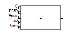
The Emax block represents an Emax or a sigmoidal Emax model, where the output is the effect level as a function of drug concentration. The baseline effect level (E0) is always zero.
The Emax block contains five input nodes and one output node.
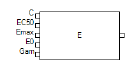
The input nodes are made available depending on the options that are selected in the Structure tab. If an input node cannot be used, it is marked with an X.
The input nodes on the Emax block can be connected to output nodes on PK compartments, observation blocks, PD blocks, and parameter blocks.
Once an output node is connected its name cannot be changed.
-
Insert an Emax block by selecting Insert > PD > Emax from the right-click menu.
To specify Emax block options
-
Use the pointer to select an Emax block.
-
In the Emx field, enter a name for the Emax block or use the default.
-
Check the Baseline checkbox if the model has a baseline response.
Selecting Baseline adds a new parameter, “first”, which has the default value E0 and is the baseline response. The Fractional checkbox is also made available. -
Check the Fractional checkbox if the Emax model is fractional.
Selecting Fractional modifies the E0 equation statement. -
Check the Inhibitory checkbox if the Emax model is inhibitory.
The structural parameters EC50 and Emax change to IC50 (concentration producing 50% of maximal inhibition) and E0 (baseline effect).
-
Check the Sigmoid checkbox if the Emax model is sigmoidal.
A new parameter, Gam, which is a shape parameter, is added. -
In each parameter field, accept the default names or type new names for each parameter.
Each parameter corresponds to an input node on the Emax block. Possible Emax parameters include:
•C: Drug concentration in plasma, or another input variable.
•EC50: Input level that achieves 50% of predicted maximum effect in an Emax model.
•IC50: Input level required to produce 50% of the maximal inhibition.
•first (E0): Baseline effect.
•EMax: Maximum drug effect.
•IMax: Maximum drug inhibition (requires that both Baseline and Inhibitory checkboxes be checked).
•Gam: Shape parameter.
The Linear block provides a simple linear model in the form of: Output=A*Input+B.
The Linear block contains four input nodes and one output node. The input nodes are made available depending on the options that are selected in the Structural tab. If an input node cannot be used, it is marked with an X.
The input nodes on the Linear block can be connected to output nodes on PK compartments, observation blocks, PD blocks, and parameter blocks. Once an output node is connected its name cannot be changed.
-
Insert a linear block by selecting Insert > PD > Linear from the right-click menu.
To specify Linear block options
-
Use the pointer to select a Linear block.
-
In the order menu, select the order of the linear model to determine how many parameters the Linear block uses.
-
In the Linear field, enter a name for the Linear block or use the default.
-
In each parameter field, accept the default names or type new names for each parameter.
Each parameter corresponds to an input node on the Linear block. Possible Linear parameters include:
•C: drug concentration in plasma, or another input variable.
•Alpha: coefficient for zero-order term.
•Beta: coefficient for first-order term (if order >=1).
•Gam: coefficient for second-order term (if order=2).
PK/PD models with stimulation or inhibition of the indirect response formation or degradation can be created using this block.
-
Insert an Indirect block by selecting Insert > PD > Indirect from the right-click menu.
The Indirect block contains five input nodes and one output node. The input nodes are made available depending on the options that are selected in the Structural tab. If an input node cannot be used, it is marked with an X.
The input nodes on the Indirect block can be connected to output nodes on PK compartments, observation blocks, PD blocks, and parameter blocks. Once an output node is connected its name cannot be changed. -
Insert an Indirect block by selecting Insert > PD > Indirect from the right-click menu.
To specify Indirect block options
-
Use the pointer to select an Indirect block.
-
In the Ind field, enter a name for the Indirect block or use the default.
-
In the Indirect menu select the indirect model type:
•Stim. Limited (limited stimulation of input)
•Stim. Infinite (infinite stimulation of input)
•Inhib. Limited (limited inhibition of input)
•Inhib. Inverse (inverse inhibition of input)
•Stim. Linear (linear stimulation of input)
•Stim. Log Linear (logarithmic and linear stimulation of input)
Use the Indirect menu options to select a model in which the response formation (build-up) or degradation (loss) is stimulated or inhibited by increased concentrations. The default response setting is the build-up of the response, or the production of the response.
-
Click Build-up multiple times to toggle between the options:
•Build-up: Changes the statement for the Ke parameter to Kin.
•Loss: Changes the statement for the Ke parameter to include Kin-Kout, where Kin is the zero-order input rate constant and Kout is the first output rate constant.
-
Click no Exponent multiple times to toggle between the options:
•no Exponent: Removes the exponent from the effect statement.
•Exponent: Adds the exponent Gamma to the effect statement.
-
In each parameter field, enter names for each parameter or use the defaults.
Each parameter corresponds to an input node on the Indirect block. Possible Indirect parameters include:
•Kin: Zero-order turnover rate for the production of a response.
•Kout: Fractional turnover rate.
•Emax: Maximum drug induced effect.
•Imax: Maximum drug induced inhibition.
•EC50: Concentration at 50% of maximal effect.
•IC50: Concentration producing 50% of maximal inhibition.
•Gam: Exponent parameter.
This block represents an effect site for a PK/PD model with a delay between the central and effect-site concentrations, that is, plots of plasma concentration versus effect level show a counter-clockwise hysteresis. See Sheiner, Stanski, Vozeh, Miller and Ham (1979). Simultaneous modeling of pharmacokinetics and pharmacodynamics: application to d-tubocurarine. Clin Pharm Ther 25:358–71 for more about modeling data with a hysteresis in the concentration-effect plot.
The Effect Compartment block contains two input nodes and one output node. The input nodes are made available depending on the options that are selected in the Structural tab. If an input node cannot be used, it is marked with an X.
The input nodes on the Effect Compartment block can be connected to output nodes on PK compartments, observation blocks, PD blocks, and parameter blocks.
Once an output node is connected its name cannot be changed.
-
Insert an Effect Compartment block by selecting Insert > PD > Effect Cpt from the right-click menu.
To specify Effect compartment block options
-
Use the pointer to select an Effect Compartment block.
-
In the Ce field, enter a name for the Effect Compartment block or use the default.
-
In the Ke0 field, enter a name or use the default of Ke0.
Ke0 is the exit rate constant from the effect compartment.
The Parameter block is used to add extra structural parameters to a model.
The Parameter block’s input nodes are labeled S1, S2, and so forth depending on how many Parameter blocks are added to the model. The output node is labeled based on the name given to the parameter.
The input node on the Parameter block can be connected to output nodes on PK compartments, observation blocks, PD blocks, and other parameter blocks. Once an output node is connected its name cannot be changed.
-
Insert a Parameter block by selecting Insert > Parameter from the right-click menu.
-
Use the pointer to select a Parameter block.
-
In the name field, type a name for the parameter.
Use Procedure blocks to write continuous functions, including differential equations, and logical statements. Within a Procedure block, functions in the Code tab are executed in the order they are listed, one or more times at each simulation step. For that reason, Procedure blocks are not suitable for counting, storing model status across time, or performing computations at specific times during simulation.
-
Insert a Procedure block by selecting Insert > Procedure from the right-click menu.
To specify Procedure block options
-
Use the pointer to select an Parameter block.
-
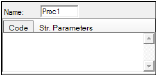
In the Name field, type a name for the procedure or use the default.
The Procedure block is labeled Proc1, Proc2, and so forth depending on how many Procedure blocks are added to the model. The output node is labeled based on the name given to the parameter. -
In the Code tab, enter any differential equations or PML (Phoenix Modeling Language) statements.
-
In the Str. Parameters tab, click Add to add a structural parameter to the Procedure block.
-
In the parameter field, type a name for the parameter.
An input node is added to the Procedure block for each new parameter that is added. -
Click the X button to remove a structural parameter.
If the statement entered in the Code tab adds a dose point to the model, then the Dosepoints tab allows users to specify if the dose point uses infusion. -
In the Dosepoints tab, check the Infusions possible? checkbox if the dose point uses infusions.
Selecting this option adds a dosing rate context to the Main Mappings and the Dosing panels.
Note:Sequence blocks cannot be entered in a procedure block when working with the graphical model. They can be entered in the textual model, however.
Each Expression block's value is set by the expression entered in the Contents tab. Note that this can only be an expression; no statements, such as assignments (using the “=” sign), or PML code can be included. An expression is any combination of numbers, identifiers, and operators representing a single value. It includes no “=” sign representing assignment.
An expression can contain:
•conditional operators (e.g., (cond) ? actionA:actionB)
•logical operators (e.g., &&, ||, !)
•comparison operators (e.g., >=, <=, !=, ==, >, <)
These are all at a lesser level of precedence than arithmetic operators. So, for example, “a+b>c” means “(a+b)>c”.
-
Insert an Expression block by selecting Insert > Expression from the right-click menu.
To specify Expression block options
-
Use the pointer to select an Expression block.
-
In the Name field, type a name for the expression or use the default.
The Expression block is labeled Expr1, Expr2, and so forth depending on how many Expression blocks are added to the model. The output node is labeled based on the name given to the parameter. -
In the Contents tab, type the expression.
-
In the Structural Parameters tab, click Add to add a structural parameter to the Expression block.
-
In the parameter field, type a name for the parameter.
An input node is added to the Expression block for each new parameter that is added. -
Click the (X) button to remove a structural parameter.
The Annotation block is used to add notes to a model.
-
Insert an Annotation block by selecting Insert > Annotation from the right-click menu.
-
Use the pointer to select an Annotation block.
-
In the Note field, type a note or description.
-
Check the Border checkbox to add a border to the annotation.
Annotation blocks do not wrap the text. -
Press ENTER to add another line to the annotation.
If the Annotation block has a border, the block can be expanded to surround the text. -
Expand the block by selecting it with the pointer.
Place the pointer over one of the blue squares on the corners of the Annotation block. Single-click and drag the blue square to expand the block around the text.
Use a vascular flow to represent blood flow in physiologically-based PK models. Use this flow to connect PK compartments representing organs or other areas into circuits of blood flow. The flow rate between organs is represented by the variable Q.
-
Insert a Vascular flow by selecting Insert > PBPK > Vascular Flow from the right-click menu.
-
Use the pointer to select the first compartment of the flow.
-
Use the pointer to select the second compartment of the flow.
Note:A Vascular Flow should connect a central or a peripheral compartment. It should not be used to connect an elimination or an absorption compartment.
To specify Vascular Flow options
-
Use the pointer to select a Vascular Flow.
-
Click Draw multiple times to toggle through the options for drawing the PK flow in the Graphical model interface.
•Diagonal: Draws the diagonal flow.
•Horizontal First: Draws the flow horizontally from the first compartment.
•Vertical First: Draws the flow vertically from the first compartment.
-
In the CL field, enter a name for the input variable or use the default.
To use the textual editor to create the structural model
•Click Edit as Textual to use PML (Phoenix Modeling Language) code to create the model.
•In the displayed dialog, click Yes to confirm using the textual editor.
When using the textual editor, the Edit as Textual button changes to either Use Builtin or Use Graphical, depending on the mode you were in before switching to the textual editor. Click this button to return to the previous mode.
The mappings panel switches to the Model panel and the model text is displayed. It represents the model as it currently exists and allows users to edit the structural model using PML code. The PML examples illustrate the use of PML to create various models and describes the use of the available statements and functions.
While typing, the text editor will provide hints for adding parameters. Type the parameter and its following comma to see the hint for the next parameter.
When in text model mode, some Phoenix Model Object option tabs change:
•The General tab displays PML errors and warnings as model code is entered in the Model panel.
•The Parameters tab displays only the parameter names. Bounds and initial values should be entered in the fixef statements in the PML code.
•The Input Options tab is where infusion information is specified.
•The Model Text tab displays only the column definition. The model code is now only displayed in the Model panel.
Note:When doing a Profile of a Textual model, avoid deleting fixef parameters as this can lead to extra copies of fixed effects appearing in the “Fixed Eff” list.
