Observations are the link between the model and the data. The model describes the relationships between covariates, parameters, and variables. The data represent a random sampling of the system that the model describes. The various types of observation statements that are available in the Phoenix Modeling Language serve to build a statistical structure around the likelihood of a given set of data.
Observation statements are used to build the likelihood function that is maximized during the modeling process. The observation statements indicate how to use the data in the context of the model.
•Count statement for Count models
•Event statement for Survival models
•LL statement for Log Likelihood models
•Multi statement for Multinomial models
•Observe statement for Normal-inverse Gaussian Residual models
•Ordinal statement for Ordinal Responses
•Observation statement action codes:
Count statement for Count models
count(observed variable, hazard expression[, options][, action code])
Similar to event, but instead of observing an occurrence variable, an occurrence count is observed. The log-likelihood is based on a Poisson or Negative Binomial distribution whose mean is the integrated hazard since the last observation. The options are:
, beta=<expression>
The presence of the beta option makes the distribution Negative Binomial, where the variance is var=mean*[1+mean*alpha^power), and alpha=exp(beta)
, power=<expression>
Power of alpha, default(1). Zero-inflation can be applied to either the Poisson or Negative-Binomial distributions, in one of two ways, by means of simply specifying the extra probability of zero, by giving the zprob argument, or by giving an inverse link function with ilink and its argument with linkp.
, zprob=<expression>
Zero-inflation probability, default(0) (incompatible with following two options)
, link=“ilogit”, “iprobit”
Or other inverse link function. If not specified, it is blank.
, linkp=<expression>
Argument to inverse link function
, noreset
When present, this option will prevent the accumulated hazard from resetting after each observation.
For the default Poisson distribution, the mean and variance are equal. If that shows inadequate variance, use of the beta option, with optional power, may be indicated. Care should be taken, since if the value of beta*power becomes too negative, that means the distribution is very close to Poisson and the Negative Binomial distribution may incur a performance cost.
Note:The Negative-Binomial Distribution log likelihood expression can generate unreasonable results for reasonable cases. For example, if count data that is actually Poisson is used, the parameter r in the usual (r,p) parameterization can become very large (and p becomes very small). The large value of r can cause a problem in the log gamma function that is used in the evaluation. So such data, which is completely reasonable, may give an unreasonable fit if care is not taken in how the log likelihood is evaluated numerically.
All about Count models
Observing a count, such as the number of episodes of vertigo over a prior time interval of one week, is also a hazard-based measurement. The simplest model of the count is called a Poisson distribution and it is closely related to the coin-toss process in the time-to-event model (discussed in “All about Time-to-Event modeling”). In this model, the mean (average) count of events is simply the accumulated hazard. One can think of the hazard as simply the average number of events per time unit, so the longer the time, the more events. Also, in the Poisson distribution, the variance of the event count is equal to the mean.
In some cases, if one tries to fit a distribution to the event counts, it is found that the variance is greater than what a Poisson distribution would predict. In this case, it is usual to replace the Poisson distribution with a Negative Binomial distribution, which is very similar to the Poisson, except that it contains an additional parameter indicating how much to inflate the variance.
Another alternative is to notice that a count of 0 (zero) is more likely to occur than what would be predicted by either a Poisson or Negative Binomial distribution. If so, this is called “zero inflation.” All of these alternatives can be modeled with the count statement.
The simplest case is a Poisson-distributed count:
count(n, h)
where n is the name of the observed variable, taking any non-negative integer value. h is the hazard expression, which can be time-varying.
To make it a Negative Binomial distribution, the beta keyword can be employed:
count(n, h, beta=b)
where b is the beta expression, taking any real value. The beta expression inflates the variance of the distribution by a factor (1+exp(b)), so if b is strongly negative, exp(b) is very small, so the variance is inflated almost not at all. If b is zero or more, then exp(b) is one or more, so the variance is inflated by an appreciable factor. The reason for encoding the variance inflation this way is to make it difficult to have a variance inflation factor too close to unity, because 1) that makes it equivalent to Poisson, and 2) the computation of the log-likelihood can become very slow.
If the beta keyword is present, an additional optional keyword may be used, power:
count(n, h, beta=b, power=p)
in which case, the variance inflation factor is (1+exp(b)^p), which gives a little more control over the shape of the variance inflation function. If the power is not given, its default value is unity.
Whether the Poisson or Negative Binomial distribution is used, zero-inflation is an option, by using the zprob keyword:
count(n, h, zprob=z)
where z is the additional probability to be given to the response n=0. Alternatively, the probability can be given through a link function, using keywords ilink and linkp:
count(n, h, ilink=ilogit, linkp=x)
where x is any real-numbered value, meaning that ilogit(x) yields the probability to be used for zero-inflation.
Count models can of course be written with the LL statement, but it can get complicated. In the simple Poisson case, it is:
deriv(cumhaz=h)
LL(n, lpois(cumhaz, n), doafter={cumhaz=0})
where cumhaz is the accumulated hazard over the time interval since the preceding observation, and n is the observed number of events in the interval. lpois is the built-in function giving the log-likelihood of a Poisson distribution having mean cumhaz. After the observation, the accumulated hazard must be reset to zero, in preparation for the following observation.
If the simple Poisson model is to be augmented with zero-inflation, it looks like this:
deriv(cumhaz=h)
LL(n, (n == 0 ? log(z+(1-z)*ppois(cumhaz, 0)):
log(1-z)+lpois(cumhaz, n)
)
, doafter={cumhaz=0}
)
where z is the excess probability of seeing zero. Think of it this way: before every observation, the subject flips a coin. If it comes up “heads” (with probability z), then a count of zero is reported. If it comes up “tails” (with probability 1-z), then the reported count is drawn from a Poisson distribution, which might also report zero. So, if zero is seen, its probability is z+(1-z)*pois(cumhaz, 0), where pois is the Poisson probability function. On the other hand, if a count n > 0 is seen, the coin must have come up “tails,” so the probability of that happening is (1-z)*pois(cumhaz, n). The log-likelihood given in the LL statement is just the log of all that.
If it is desired to use the link function instead of z, z can be replaced by ilogit(x). (There are a variety of built-in link functions, including iloglog, icloglog, and iprobit.)
If the Negative Binomial model is to be used, because Poisson does not have sufficient variance, in place of:
lpois(cumhaz, n)
the expression:
lnegbin(cumhaz, beta, power, n)
is used instead, where the meaning of beta and power are as explained above. If beta is zero, that means the variance is inflated by a factor of two. Typically, beta would be something estimated. If it is not desired to use the power argument, the default power of one should be used.
Event statement for Survival models
event(observed variable, expression [, action code])
Specifies an occur observed variable, which has two values: 1, which means the event occurred, or 0, which means the event did not occur. The hazard is given by the expression.
The event statement creates a special hidden differential equation to accumulate, or integrate, the hazard rate, which is defined by the expression in the second argument. This integration is reset whenever the occur variable is observed, so the integral extends from the time t0 of the previous occur observation to t1, the time of the current observation. Let cum_hazard=integral of the hazard during the period [t0,t1]:
cum_hazard= .
.
Then the probability that an event will not occur in the period is: S=exp(-cum_hazard). Therefore, if the period terminates with an observation occur=0 at t1, the likelihood is S. If the period terminates at t1 because an event occurred at time=t1 (occur=1), then the likelihood is S*hazard(t1), where hazard(t1) is the hazard rate at t1. These likelihood computations are performed automatically whenever an occur observation is made.
Note:The observations of 0 (no event) can occur at pre-defined sampling points, but observations of 1 (event occurred) are made at the time of the event.
Event models are inherently time based, and require a mapping for a time value.
All about Time-to-Event modeling
Consider a process modeled as a series of coin-tosses, where at each toss, if the coin comes up “heads,” that means an event occurred and the process stops. Otherwise, if it comes up “tails,” the coin is tossed again. The graph below shows that process if the probability of “heads” is 0.1, and the probability of “tails” is 0.9.
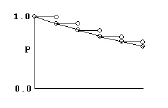
It is easy to see that the probability of getting to time 5 without getting a “heads” is 0.9 multiplied by itself 5 times. Similarly, the probability of getting a “heads” at time 5 is 0.1 multiplied by the probability of getting to time 4 without getting “heads” or 0.94*0.1.
To put it in symbols, if the probability of “heads” is p, then the probability of “heads” at time n is:
(1 – p)(1 – p) … n – 1 times … (1 – p) p
Since in model fitting the log of the probability is desired, and since, if p is small, log(1 – p) is basically –p, it can be said that the log of the probability of “heads” at time n is:
–p –p … n – 1 times … –p+log(p)
Note that p does not have to be a constant. It can be different at one time versus another.
The concept of “hazard,” h, is simply probability per unit time. So if one cuts the time between tosses in half, and also cuts the probability of “heads” in half, the process has the same hazard. It also has much the same shape, except that the tossing times come twice as close together. In this way, the time between tosses can become infinitesimal and the curve becomes smooth.
If one looks at it that way, then the probability that “heads” occurs at time t is just:
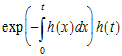
where the exponential part is the probability of no “heads” up to time t, and h(t) is the instantaneous probability of “heads” occurring at time t. Again, note that hazard h(t) need not be constant over time. If h(t) is simply h, then the above simplifies to the possibly more familiar:

The log of the probability is:
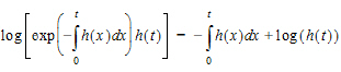
In other words, it consists of two parts. One part is the negative time integral of the hazard, and that represents the log of the probability that nothing happened in the interval up to time t. The second part is the log of the instantaneous hazard at time t, representing the probability that the event occurred at time t. (Actually, this last term is  as a protection against the possibility that h(t) is zero.)
The event statement models this process. It is very simple:
event(occur, h)
where h is an arbitrary hazard function, and occur is the name of an observed variable. occur is observed on one or more lines of the input data. If its value is 1 on a line having a particular time, that means the event occurred at that time, and it did not occur any time prior, since the beginning or since the time of the prior observation of occur.
If the observed value of occur is 0, that means the event did not happen in the prior time interval, and it did not happen now. This is known as “right censoring” and is useful to represent if subjects, for example, withdraw from a study with no information about what happens to them afterward. It is easy to see how the log-likelihood of this is calculated. It is only necessary to omit the log(h) term.
Other kinds of censoring are possible. If occur equals 2, that means the event occurred one or more times in the prior interval, but it is not known when or how many times. If occur is a negative number like -3, that means the event occurred three times in the prior interval, but it is not known when. There is a special value of occur, -999999, meaning there is no information at all about the prior interval, as if the subject had amnesia. These are all variations on “interval censoring.” The log-likelihoods for all these possibilities are easily understood as variations on the formulas above.
This can be done with the log-likelihood (LL) statement instead, as follows:
deriv(cumhaz=h)
LL(occur, -cumhaz+occur*log(h), doafter={cumhaz=0})
The deriv statement is a differential equation that integrates the hazard. The LL statement says that variable occur is observed and it is either 1 (the event occurred) or 0 (it did not occur). It gives the log-likelihood in either case. Then, after performing the observation, the accumulated hazard is set to zero. This allows for the possibility of multiple occurrences.
LL statement for Log Likelihood models
LL(observed_variable, expression[, simulate={simulation_code}]
[, action code])
This statement specifies there is an observed variable, and when it is observed, its log-likelihood is the given expression. Optional action code is executed before or after the observation. If the “simulate” keyword is present, then during simulation or predictive check, the simulation code can assign a value to the observed variable.
The following is an example of a time to event model, illustrating how simulate can work on the LL statement.
covariate(DOSETOT,cycledays,uni01,timeforhistograms)
deriv(E=Kin*DOSETOT/cycledays-Kout*E)
sequence{E=E0}
real(u, i, prob)
LL(EObs
,-E+EObs*log(E)-lgamm(EObs+1)
, simulate={
u=unif()
prob=0
i=0
prob=prob+exp(-E+i*log(E)-lgamm(i+1))
while(u >= prob){
prob=prob+exp(-E+i*log(E)-lgamm(i+1))
i=i+1
}
EObs=i
}
)
In the example above, EObs is the observed variable and -E+EObs*log(E) -lgamm(EObs+1) is the expression. The optional action follows the simulate keyword. It is separate from the last action code [, action code] (e.g. [,doafter={E=0}]).
Multi statement for Multinomial models
multi(observed variable, inverse link function(, expression)*
[, action code])
This statement specifies an integer-valued categorical observed variable. The name of an inverse link function is given, such as ilogit. The next part of the statement is a series of offset expressions in ascending order, such as C-X01 or C-X12, where X01 is the value of C that evenly divides the response between zero and one, and X12 divides the response between one and two.
This relationship between offset expressions is illustrated below, but without using a variable in the expression. The domain of the parameters X01 and X12 exists along the unbounded real line. The goal is to divide the range of the inverse function (0,1) into the probabilities of the categorical observations. This preserves the constraint that the sum of the probabilities equals one.
In the illustration below, the first breakpoint, proceeding from left to right, is X01. The value of the inverse function (ilogit, in this case) is taken at X01 and P0, which is the probability of the first category, is P0=ilogit(X01). The next breakpoint is X12, and the probability of observing the second category is P1=ilogit(X12)-ilogit(X01), which is the cumulative probability between the first and second breakpoints. The third observation has probability P2=1-P0-P1, which is the remainder of the cumulative probability.
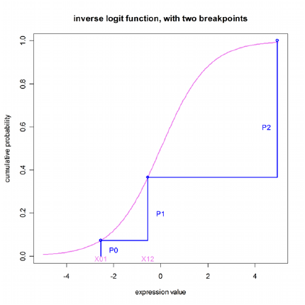
Relationship between offset expressions
It is simple to extend the example beyond simple values of X01 and X12, to include a function of covariates. Given the relationship between the category probabilities and the probabilities, it is easy to why the initial estimates of the parameters should be given in such a way as to not cause the computed values of any of the probabilities to be negative. It is imperative that initial conditions be chosen carefully to ensure convergence.
All about Multinomial (ordered categorical) responses
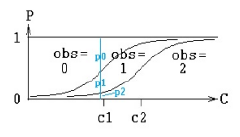
Consider a model in which an observation can take values zero, one, and two. No matter what value concentration C is, any value of the observation is possible, but C affects the relative probabilities of the observed values. If C is low, the most likely observation is zero. If it is high, the most likely observation is two. In the middle, there is a value of C at which an observation of one is more likely than at other values of C.
The following figure illustrates the concept. At any value of C, there is a probability of observing zero, called p0. Similarly for one and two. The probability is given by the inverse of a link function, typically logit. In this picture, there are two curves. The left-hand curve is ilogit(C-c1) and it is the probability that the observation is ³1. The right-hand curve is ilogit(C-c2), and it is the probability that the observation is ³2. The probability of observing one (p1) is the difference between the two curves. When doing model-fitting, the task is to find the optimum values c1 and c2. Note that c2 is the value of C at which the probability of observing two (p2) is exactly 1/2, and that c1 is the value of C at which the probability of observing a value greater than or equal to one (p1+p2) is exactly 1/2. Note also that c1 and c2 have to be in ascending order, resulting in the curves being in descending order.
There are statements in PML for modeling such a response: multi, and ordinal, and it can also be done with the general log-likelihood statement, LL. The multi statement for the above picture is this:
multi(obs, ilogit, C-c1, C-c2)
obs is the name of the observed variable, ilogit is the inverse link function, and the remaining two arguments are the inputs to the inverse link function for each of the two curves. Since c1 and c2 are in ascending order, the inputs for the curves, C-c1 and C-c2, are in descending order.
A more widely accepted way to express such a model is given by logistic regression, as in:
P(obs >= i)=ilogit(b*C+ai)
where b is a slope (scale) parameter, and each ai is an intercept parameter. The ordinal statement expresses it this way:
ordinal(obs, ilogit, C, b, a1, a2)
where the ai are in ascending order. This is equivalent to the multi statement:
multi(obs, ilogit, -(b*C+a1), -(b*C+a2))
where, since the ai are in ascending order, the arguments -(b*C+ai) are in descending order, as they must be for the multi statement.
To do all this with the log-likelihood statement (LL) requires calculating the probabilities oneself, as shown below. Using the original parameterization with c1 and c2:
pge1=ilogit(C-c1)
pge2=ilogit(C-c2)
LL(obs, obs==0?log(1-pge1):
obs==1?log(pge1-pge2):
log(pge2\0)
)
The first statement computes the first curve, the probability that the observation is greater than or equal to one, pge1. The second statement computes the second curve, the probability that the observation is greater than or equal to two, pge2. Note that these are in descending order, because the probability of observing two has to be less than (or equal to) the probability of observing one or two.
The third statement says obs is the observed variable, and if its value is zero, then its log-likelihood is the log of the probability of zero, where the probability of zero is one minus the probability of greater than or equal to one, i.e., log(1-pge1). Similarly, if the observation is one, its probability is pge2-pge1. Note that since pg1e>pge2, the probability of one is non-negative. Similarly, if the observation is two, its probability is pge2-pge3, where pge3 is zero because three is not a possible observation.
If, on the other hand, one were to use the typical slope-intercept parameterization from logistic regression, the first two lines of code would look like this:
pge1=ilogit(-(b*C+a1))
pge2=ilogit(-(b*C+a2))
and the LL statement would be the same.
Observe statement for Normal-inverse Gaussian Residual models
observe(observedVariable([independentVariable])=
expression[, bql][, action code])
The above statement specifies that the observedVariable is a function of some prediction and some Gaussian error. The bql option specifies that a lower limit of quantification can be applied to this observation, allowing for occurrence observations to be included.
If action code is given, that indicates actions to be performed before or after each observation. If there are no differential equations, the independentVariable for the observations can be specified. This allows the Phoenix Model object to produce the appropriate output plots and worksheets.
For example, a Michaelis-Menten model of reaction kinetics can be written as:
observe(RxnRate (C)=Vmax*C/(C+Km)+eps)
Ordinal statement for Ordinal Responses
ordinal(observedVariable, inverseLinkFunction,
explanatoryVariable, beta, alpha0, alpha1, …)
For example:
ordinal(Y, ilogit, C, slope, intercept0, intercept1, …)
where the intercepts are in numerically ascending order. It fits the model:
P(Y ? i | C)=ilogit(C*slope+intercepti)
And if there are m values of Y, they are 0, 1, … m – 1, and there are m – 1 intercepts.
This is equivalent to the multi statement:
multi(Y, ilogit, -(C*slope+intercept0), -(C*slope+intercept1), …)
Observation statement action codes:
Action codes may be given, within an observation statement, which specify computations to make either before or after an observation is made. For instance, if there is a urine compartment that is emptied at each observation, part of the model may resemble this:
deriv(urineVol=gfr)
deriv(urine_amt=gfr*Cp*fu)
observe(Uvol=urineVol+epsUv, doafter={urineVol=0})
