Running NLME Engines in Command Line Mode
The Phoenix Modeling Language (PML) supports model building through a text-based modeling language that allows users to describe, fit, and simulate models.
The PML language supports specification of input and/or output data, trial related settings such as dosing and treatment sequence, as well as flexible model definitions for PK/PD and general Nonlinear Mixed Effects (NLME) modeling including survival analysis and modeling of categorical responses.
PML includes the necessary structures for seamless integration of modeling with trial simulation and related analyses. PML draws on established practices in S-PLUS and NONMEM to make PML user-friendly for people familiar with those software packages.
Users do not need to have Phoenix running in order to run PML models from the command line. When Phoenix is installed, the files necessary to run PML models from the command line are also installed.
This section covers the following topics, describing how to operate the NLME engine in Windows command line mode using batch scripts named RunNLME.bat and RunNLMEMPI.bat.
Running PML models from the command line requires the following:
•An NLME license and a PML license
•Phoenix Platform/WinNonlin 8.1
•MinGW (Minimalist GNU for Windows) C++ compiler
For more on MinGW, see the MinGW Web site. MinGW is installed during the Phoenix installation process. Only the version of MinGW that comes with the Phoenix installation package is guaranteed by Certara to be compatible with Certara software.
•Two Ghz. Intel-compatible CPU
•Four gigabyte RAM minimum, but eight gigabytes is recommended
•300 megabytes free harddrive space
PML and multi-processor or multi-core computers
PML supports parallel processing through the use of the Message Passing Interface (MPI). Use the RunNLMEMPI.bat batch file to run models using multiple processors or processor cores.
Users with multiple processor or multiple-core computers can install MPICH2, a free and portable implementation of the Message Passing Interface. MPICH2 is also available for installation as part of the Phoenix installation process during Complete Installation or can be selected during Custom Installation. Or users can install MPICH2 themselves using the mpich2-1.4.1p1-win-x86-64.msi installer, which is included with the Phoenix installation package.
For more on MPICH2, visit the MPICH2 Web site.
Installing MPICH2 is optional, and is not necessary for computers with one processor or one processor core.
Install the executables and examples
Run the setup.exe installation program that comes with the Phoenix installation package. For more on installing Phoenix, see “Phoenix Installation and Licensing”.
This installs the executables, DLLs, and C++ files needed to run the NLME engines in command line mode into <Phoenix_install_dir>\application\lib\NLME\Executables.
A group of seven modeling examples are installed in separate subfolders in <Phoenix_install_dir>\application\Examples\NLME\Command Line. You can save a copy of the Examples directory (installed with Phoenix) to your Phoenix project directory via the Project Settings in the Phoenix Preferences dialog.
In addition to the model, column definition, and data files, each example folder includes three batch files: Cmd.bat, RunNLME.bat, and RunNLMEMPI.bat.
Note:The Command window used to execute the command line scripts must be Run as Administrator. If running on a server, the user must be logged in as an administrator.
Run the example model 1:
-
Navigate to …\Examples\NLME\Command Line\Model 1.
-
Double-click the file Cmd.bat, or right-click to Run as Administrator.
A Windows command line window is opened. -
In the command window, navigate to the Model 1 subdirectory.
-
Run 500 iterations using engine 3 (-LB) on model lyon04.mdl with the column mapping file COLS04.txt and the data file EMAX02.csv with this command:
RunNLME 3 500 lyon04.mdl COLS04.txt EMAX02.csv
The output is created in the Model 1 subdirectory.
Run example models 2–7:
-
Select the Model 2 subdirectory.
-
Double-click the file Cmd.bat, or right-click to Run as Administrator.
-
In the command window, navigate to the Model 2 subdirectory.
-
Run 500 iterations using engine 3 on model lyon05.mdl with the column mapping file COLS05.txt and the data file EM01.csv with the command:
-
To run the models 3–7, open each model subdirectory and double-click Cmd.bat, or right-click to Run as Administrator.
-
Use the following statements to run each model from the command line:
RunNLME 3 500 lyon05.mdl cols05.txt em01.csv
Model 3:
RunNLME 5 200 fm1theo.mdl colstheo.txt ThBates.csv
Model 4:
RunNLME 5 200 fm3theo.mdl colstheo.txt ThBates.csv
Model 5:
RunNLME 5 200 pheno2.mdl colspheno2.txt pheno2.csv
RunNLME 5 200 pheno2.mdl colspheno2.txt phobs.csv
Model 6:
RunNLME 5 200 apolipo.mdl colsapolipo.txt apo2.csv
Model 7:
RunNLME 5 200 apolipo2.mdl colsapolipo.txt apo2.csv
Note:The Command window used to execute the command line scripts must be Run as Administrator.
The NLME command line statement has a basic syntax that is composed of six command line arguments.
runNLME engine_number maxiterations model colmap data
where:
•runNLME: The name of the batch file used to call the compiler to compile the model, in this case, the file is called runNLME.
•engine_number: The number corresponding to the specific engine to use with the model.
1: QRPEM (Quasi-Random Parametric expectation-maximization)
2: IT2S-EM (Iterated 2-stage expectation-maximization)
3: FOCE L-B (First-Order Conditional Estimation, Lindstrom-Bates)
4: FO (First Order)
5: General likelihood engine, which includes FOCE ELS (Extended Least Squares; default), Laplacian, and adaptive Gaussian quadrature methods. Method selection is controlled by flags and parameters in file nlmeflags.asc.
6: Naïve pooled
•maxiterations: An integer between zero and 10000 that specifies the maximum number of iterations to run the main optimization routine in each engine. If maxiterations is zero, no optimization is run but the model is evaluated at the initial solution defined in the model file or restart file. In this case, the standard output files are written using the initial solution as the fitted solution. Any post optimization computations such as a nonparametric analysis or a standard error computation specified in nlmeflags*.asc are also run.
•model: Name of the model file.
•colmap: Name of a column mapping file that associates variable names in the model file with column names in the data file. Use of quotes in this file is optional to allow otherwise non-permitted column names to be resolved.
•data: Name of the data file.
For example,
runNLME 3 200 lyon04.mdl COLS04.txt EMAX02.csv
runs the FOCE L-B engine (engine number 3) on model file lyon04.mdl with the column mapping file COLS04.txt and the data file EMAX02.csv for a maximum of 200 iterations.
|
File |
Purpose |
|
model file |
mandatory command line argument 4 |
|
colmap file |
mandatory command line argument 5 |
|
data file |
mandatory command line argument 6 |
|
nlmeflags.asc |
optional control file |
|
logrestart.asc |
optional restart file |
The three mandatory input files are always designated in the command line.
An optional fourth control input file called nlmeflags.asc is used to set certain environmental flags and tolerances to values other than the default values. If this file is not present in the command line arguments, then the environmental flags and tolerances are set to their default values. The file is created with every modeling run.
The format and default values of the nlmeflags.asc file are listed below. Every successful run of the NLME engine creates a lognlmeflags.asc file which contains flags and values that can be copied to the nlmeflags.asc file.
Copy the text from lognlmeflags.asc to nlmeflags.asc and change the applicable values in order to create and use nlmeflags.asc file in a modeling run.
The optional fifth command line argument input file is called logrestart.asc. It is used to designate an initial starting solution other than that specified in the model file. Every successful run of the NLME engine creates a logrestart.asc file which can then be used to initialize later runs.
The flag for controlling whether or not to use logrestart.asc is in the !iflagrestart line in nlmeflags.asc.
Example usage for the command line arguments:
RunNLME 5 500 lyon04.mdl COLS04.txt EMAX02.csv nlmeflags.asc logrestart.asc
The lognlmeflags.asc control file
The standard lognlmeflags.asc control file consists of 11 lines with standard default values specified as entries. The following lines are typical contents of a lognlmeflags.asc file:
0 !iflagnp (0=do not run, otherwise # of nonparametric generations)
0 !iflagrestart (0=no, 1=start from solution in logrestart.asc)
1 !norderAGQ
1 !iflagfocehess (1=foce, 0=Laplacian numerical Hessian)
1 !iflagverbose (verbose mode is always used)
0 !iflagstderr (0=none, 1=central diff, 2=forward diff)
1 -1 !METHODblup, NDIGITblup (expert usage, do not change)
1 7 !METHODlagl, NDIGITlagl (expert usage, do not change)
0.100E-02 !tolmodlinz (step size for model linearization)
1 !iflagIEXP (1=secant, 0=hessian)
0.100E-01 !tolstderr (step size for standard error computation)
0 !nrep_pcwres (0=do not run, otherwise # of replicates)
0 !npresample (not currently used)
0 !niter_mapnp (0=do not run, otherwise # of MAP_NP iterations)
Note:If the nlmeflags.asc control file is not used then the default values are used. The file lognlmeflags.asc logs which values were used in a modeling run.
The control flags include:
-
!iflagnp: Controls whether and how intensively to run a nonparametric analysis after the initial parametric analysis is run.
•If iflagnp=0, no nonparametric analysis is run.
•If iflagnp>0, iflagnp designates the number of generations to run in the evolutionary nonparametric algorithm.
•If iflagnp=1, optimal probabilities on support points placed at the parametric post hoc estimates are computed.
•If iflagnp>1, support point positions are also optimized, but this can be computationally intensive. The output of probabilities and support points is sent to the file nparsupport.asc.
-
!iflagrestart: Specifies the source of the initial solution.
•If iflagrestart=0, the initial solution consists of the starting values in the model file.
•If iflagrestart=1, the initial solution is read from the logrestart.asc file, which is created during a previous run of the same model.
-
!norderAGQ: Only applicable to engine five, and is ignored for other engines. This flag designates the number of adaptive Gaussian quadrature (AGQ) points along each random effects dimension. The maximum value=40, but note that the total number of quadrature points is norderAGQ^(number of random effects), so it is best practice to use a small integer, unless the number of random effects is one.
•If norderAGQ=1, this corresponds to the Laplacian approximation.
•If norderAGQ>1, then adaptive Gaussian quadrature is used.
Exceptions:
•If norderAGQ=1 and iflaghess=1, then the FOCE ELS (Extended Least Squares) objective function is used, which is similar to NONMEM FOCE.
•If norderAGQ=1 and iflaghess=0, then the Laplacian objective function is used, which is similar to NONMEM Laplacian objective function.
•norderAGQ>1 and iflaghess=1 creates an adaptive Gaussian quadrature with a Gaussian kernel defined by the FOCE approximation.
•norderAGQ>1 and iflaghess=0 creates an adaptive Gaussian quadrature with a Gaussian kernel defined by a numerical differentiation Hessian approximation.
-
!iflagfocehess: Controls how the Hessian matrix is approximated.
•If iflagfocehess=1, the FOCE L-B approximation to compute the approximation to the Hessian matrix of the joint log likelihood function for each individual.
•If iflagfocehess=0, the Hessian matrix is approximated by numerical differentiation.
-
!iflagverbose: This value is always set to 1, so verbose mode always used.
-
!iflagstderr: Controls the standard error computation.
•If iflagstderr=0, then no standard error computation is attempted.
•If iflagstderr=1, a standard error computation with central differences for the required second derivatives of the log likelihood is attempted. This is much more computationally intensive but more accurate than forward differences.
•If iflagstderr=2, forward differences are used.
•If iflagstderr>0, then the relative step size to be used is specified in !tolstderr.
-
!METHODblup: Expert usage only. This flag specifies the optimization method (1=line search, 2=dogleg, 3= Levenberg-like trust region) to be used in the OPTIF9 routine for optimization of the “blups,” which are post hoc estimates or modes of the joint likelihood function for each individual. It is best practice to not deviate from the default.
-
NDIGITblup: Expert usage only. This is an input of the estimate of the available accuracy of the OPTIF9 blup objective function in terms of decimal places. It is best practice to not deviate from the default.
-
!METHODlagl: Similar to !METHODblup, but applicable to the OPTIF9 optimization of overall likelihood function in engine five. It is not suggested to deviate from the default.
-
NDIGITlagl: Similar to NDIGITblup, but applicable to the OPTIF9 optimization of overall likelihood function in engine five. It is best practice to not deviate from the default.
-
!tolmodlinz: Relative step size to use in numerical differentiation of the model function for FOCE L-B linearization.
-
!iflagIEXP: Specifies whether calculation of the likelihood function is too expensive or not to calculate.
•If iflagIEXP=0, then the overall quasi-Newton optimization step assumes that the likelihood function is not too “expensive” to evaluate and a numerical Hessian matrix is used for the Newton step.
•If iflagIEXP=1, the overall likelihood function is assumed to be too “expensive” to evaluate, which is almost always true for NLME estimation problems, and a secant approximation is used. It is suggested that you always use iflagIEXP=1.
-
!tolstderr: Relative step size to use in differentiation of log likelihood function for computation of standard errors.
-
!nrep_pcwres: Controls whether or not the simulation based PCWRES statistic is computed in the residuals table. If nrep_pcwres=0, the statistic is not computed. Otherwise, it is computed using nrep_pcwres simulation replicates (maximum of 1000).
-
!npresample: Not currently used.
-
!niter_mapnp: Controls whether or not the MAP_NP procedure for improving initial fixed effect guesses is used. If niter_mapnp=0, this option is not used. Otherwise, it is used for niter_mapnp iterations (a reasonable value to use is niter_mapnp=3).
Running QRPEM in command line mode
The numerical engine code for the QRPEM engine is 1, so a typical command line invocation of QRPEM with model file test.mdl, column mapping file cols1.txt, data file data1.txt, and a maximum iteration limit of 200 takes the form:
runnlme.bat 1 200 test.mdl cols1.txt data1.txt
The output files for QRPEM are the same as for the other engines.
In addition to the standard engine controls that can be provided in the file nlmeflags.asc discussed previously (see “The lognlmeflags.asc control file”) and which generally apply to all engines, there are some QRPEM-specific controls that apply only to the QRPEM engine and that are passed in a simple text file qrpemflags.asc.
Note:In UI mode, these controls are set in the Run Options tab.
As with nlmeflags.asc, if the qrpemflags.asc file is omitted, the default values of the various QRPEM controls will be used. However, if the user wants to override any of the QRPEM default control values, the qrpemflags.asc file must be provided in the current active directory (typically the directory containing the model, mapping, and data files). A sample qrpemflags.asc file containing default values of the controls is shown below and is also provided in …\Examples\NLME\Command Line.
300 !Nsamp number of eta samples per subject
0 !impsamptype type of importance sampling
0 !impmapflag 0=no MAP assist after first iteration,
1=MAP step on every iteration
0 !iflagmcpem 0=QRPEM sampling, 1=MCPEM sampling
1 !iflagscramble 0=none, 1=Owen, 2=Faure-Tezuka
10 !NSIR sample size for estimating fixed effects
not associated with random effects
0.1d0 !acceptance ratio
0 !irunall if irunall=1, all iterations will be run,
regardless of convergence behavior
0 !Nburn number of burn in iterations
0 !ifreezeOmega freeze Omega during burn-ins flag (0=no, 1=yes)
0 !ipostrestart posterior restart flag: 0=no,
1=use posteriors from previous run if available
! end qrpemflags.asc
The QRPEM control flags include:
-
Nsamp: The number of samples used to evaluate the posterior mean and covariance integrals for each subject. Increasing this value will improve the accuracy of the integrals and the likelihood evaluation, and generally will result in better (closer to the true maximum likelihood values) parameter estimates, but will also increase execution time. The maximum permissible value is 30000.
-
impsamptype: Specifies the importance sampling type:
•impsamptype= –2: Use a defensive Gaussian mixture with 2 components.
•impsamptype= –3: Use a defensive Gaussian mixture with 3 components.
•impsamptype=0: Use a standard Gaussian distribution (no mixture), also referred to as multivariate normal (MVN).
•impsamptype=1: Use a multivariate Laplace distribution (MVL). The MVL distribution has fatter tails than the corresponding normal distribution with the same mean and covariance matrix.
•impsamptype=2: Use a direct sampling, which means to sample directly from the N(0,Omega) population distribution, and not use any importance sampling at all.
•impsamptype > 2: Use a multivariate T (MVT) with impsamptype degrees of freedom. A value within the general range of four to 10 is recommended if an MVT distribution is desired. Any values larger than this are not significantly different than the MVN distribution and will be inefficient relative to simply using MVN. The T distribution has fatter tails that decay more slowly than the corresponding MVN distribution. The MVT decay rate is governed by the degrees of freedom: lower values correspond to slower decay and fatter tails.
The rationale for using MVL or MVT is to increase the sampling frequency from the target posterior distribution tails in case that distribution has more slowly decaying tails than that of a multivariate normal distribution. An alternative to using MVL or MVT to accomplish this is to use a lower value of acceptance ratio, as discussed below.
-
iflagmcpem: A binary 0/1 flag.
•Default=0 or off.
•If set to 1, QR sampling is turned off and replaced by Monte Carlo random sampling. This may be of interest for pedagogical purposes or if the most direct comparison possible is desired with other MCPEM algorithms such as those found in NONMEM 7 or S-ADAPT. However for production runs, using the default setting MCPEM=0 is strongly recommended to get the speed and accuracy advantages of QR sampling.
-
iflagscramble: A numeric selector that determines whether and what type of ‘scrambling’ is used. The possible values are 0 (no scrambling), 1 (Owen scrambling, the default), and 2 (Faure-Tezuka scrambling). Scrambling is a technique that de-correlates the components of the quasi-random sequence, making it look more random, without affecting the basic low discrepancy property that improves the accuracy of QR relative to random sampling for numeric integration. In some cases, use of scrambling can further improve the numerical accuracy of the integrals relative to a basic non-scrambled QR sequence.
-
NSIR: Samples is an integer value (default=10) that determines the number of Sampling-Importance-Resampling points/per subject to include in the nonlinear log likelihood optimization that is used to estimated fixed effects that appear in nonlinear covariate models, residual error models, and any instance of a fixed effect that is not paired with a random effect in a structural parameter definition. Increasing # SIR samples will improve the accuracy of these estimates but at higher computational cost. The total number of samples is the product of # SIR samples and the number of subjects. Thus with 100 subjects and the default value of # SIR samples=10, a total of 1000 samples is used, which is usually more than adequate. Normally # SIR samples should only be increased if the number of subjects is small. The maximum value of # SIR samples is ISAMPLE, the total number of sample points per subject.
-
acceptance ratio: A real valued (default=0.1) parameter that controls the ratio g of the covariance matrix of the importance sampling distribution to the estimated covariance matrix of the underlying posterior distribution through the formula:
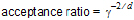
where d is the number of random effects. To insure an adequate sampling in the tails of the target posterior distribution, a g > 1, corresponding to acceptance ratio < 1, is desired. Decreasing the acceptance ratio increases g and widens the tails of the importance sampling distribution. However, if this is taken too far, the sampling becomes very inefficient since most sample points will lie in the tails far from the highest likelihood region and hence will be uninformative. Note that as an alternative to decreasing acceptance ratio, one of the fatter tail distributions MVL or MVT can be used.
-
irunall: A binary (0 or 1) flag that, if set to 1, will cause all iterations that are requested on the command line to be run. If irunall is set to its default value of 0, then iterations will be run until either a) convergence is achieved, or b) the maximum number of iterations is hit. Thus setting irunall in effect turns off application of the convergence criterion.
-
Nburn: An integer that specifies how many burn in or preconditioning iterations are performed before actual optimization steps are attempted. During these burn in iterations, only internal parameter values related to the estimated means and covariances of the posteriors are changed, but no changes are made to fixed or random effect parameter estimates. Generally, burn in iterations are only necessary when evaluating the log likelihood at the initial estimate (this is done by specifying zero iterations in the command line iteration limit), in which case about 15 burn in iterations are usually adequate. During the burn in process, the reported log likelihood value at the starting point will converge to an accurate estimate of the actual log likelihood at that point. The default setting is zero burn in iterations.
-
ifreezeomega: Modifies the meaning of Nburn. If ifreezeomega=1, then Omega is frozen during the burn in iterations.
-
ipostrestart: The posterior restart flag.
•If ipostrestart=0, restart is not used.
•If ipostrestart=1, the final posterior means and covariance matrices from the immediately preceding run are used to initiate the current run.
