PK Model parameters are grouped into categories:

-
Select the Number of Compartments from the pulldown.
One central compartment and up to two peripheral compartments can be added. For each peripheral compartment added, two parameters are also added to the model to account for the flow between the compartments. -
Select the Elimination equation to use from the pulldown:
-
Select the method of drug delivery from the Administration-Absorption pulldown:
Intravenous or First-Order -
Check the Time Lag box to add a time delay parameter to the model.
Adding a time lag assumes that there is a fixed amount of time between drug delivery (dose time) and when the drug is introduced into the blood.
–Linear: Elimination is linear.
–Michaelis-Menten: Converts the model to a saturable elimination model (Michaelis-Menten kinetics). A saturable model uses two parameters:
Km: Concentration to achieve half of maximal metabolic rate.
Vmax: The maximum metabolic rate.
Press Options to expand and contract the display of additional settings available for the model.
-
Use the Parameterization pulldown to select the type of parameterization for the model.
-
For Micro or Clearance parameterization, check the Closed form box to convert the model from a differential equation model to a closed-form algebraic model.
The closed-form model runs faster, but has some disadvantages: -
Check the Infusion box if the model uses a constant rate of drug delivery.
Infusions can be selected for intravenous and extravascular input. If checked, a Duration checkbox is displayed for changing from infusion rate (unchecked) to infusion duration (checked). -
Check the Elimination Compartment box if urine is being analyzed or data is available for any type of elimination compartment.
Selecting this option adds a differential equation for A0, the amount of a drug excreted from the body. An elimination compartment is added to the model and included in the model code as a urinecpt statement.
Adding an elimination compartment to a Clearance model removes the Closed form option and adds the Fraction Excreted Parameter option for toggling the inclusion of the fraction excreted parameter.
–Micro: Expresses the model as differential equations having mass transfer rate constants associated with a compartmental model. Adds the mass transfer rate parameters, such as Ke, the rate of elimination, and writes the derivatives in terms of compartmental masses.
–Clearance: Expresses the model as differential equations having clearances associated with a compartmental model. Adds the inter-compartmental clearance parameters, such as Cl, the clearance rate.
–Macro: Expresses the model as a closed-form sum of exponentials. This option directly models concentration in the central compartment. Primary parameters are the sum of exponential terms that model concentration in the central compartment. Volume is not in the model but can be derived as a secondary parameter. Since Macro models use concentration, an assumption must be made about the size of a reference initial dose, called a “stripping dose”. The user can enter the dose (A1) as well as a stripping dose (A1Strip). If no stripping dose is mapped, the stripping dose is assumed equal to the dose.
A note about stripping dose: The Macro model has a sum of exponentials that are fitted to the original observed value of C, using some original dose. If the model is again fitted against data obtained at another time with a higher or lower dose, then the question is how to make the model predict higher or lower values of C. This is done by multiplying the model's predicted value of C by a ratio of the current dose and the original dose. The value used for the original dose is called the “stripping dose”, and it allows the model to be used with dose values and sequences different from the original.
–Macro1: Model is expressed as a closed-form sum of exponentials. This option models the amount in the central compartment (A) and Volume is a primary parameter. Primary parameters are the sum of exponential terms plus the parameter Volume. The amount in the central compartment is modeled as a sum of exponentials and then the Volume parameter is used to convert that amount to a concentration.
–There can only be one observed variable.
–The differential system being converted must be linear.
–Any covariates used in the model must be constant for the duration of the observations.
-
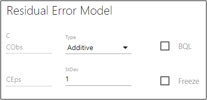
In the first field below C, type the name of the observed quantity variable (e.g., CObs).
-
In the second field below C, type the name of the epsilon variable (e.g., CEps).
The epsilon variable represents a normal error with standard deviation as specified in the stdev field. -
In the StDev field, type a value for the standard deviation.
-
Check the BQL box if the dataset contains BQL values for the observation data.
When checked, the engine automatically reverts to the Laplacian method.
A worksheet with a censored column CObsBQL can be used as the input for a model with the option BQL. If BQL is selected, a column can be mapped to the CObsBQL context. This column can contain two categories of values: non-zero number (censored) or zero/blank (non-censored). A concentration value marked as censored (CObsBQL<>0 and it is not empty) means that the true value of the observation is unknown, but it is not greater than the observed value (e.g., LLOQ, which is provided in the CObs cell for that row) and then the cumulative distribution function for the normally distributed error is used to calculate the likelihood. (The likelihood is the probability of falling into the interval between minus infinity and LLOQ, where LLOQ is given the value of the CObs or EObs column on that row.) If a concentration value is flagged as non-censored, then the probability density function is used to calculate the likelihood.
The context name CObsBQL changes based on what is typed in the observed quantity variable field. For example, instead of CObsBQL, it could be ConcBQL. -
When BQL is checked, the Static LLOQ switch becomes available. Turn the switch on to enter a numeric value of LLOQ (>0) in the displayed field.
In the event that CObsBQL is not mapped to a column in the dataset, then the static value of LLOQ will be used, so any observed value less than or equal to that LLOQ value is treated as censored. If a value is specified and the CObsBQL column (or other column with a BQL flag) is mapped, the value in the observation column will be used as the LLOQ and will override the static LLOQ. -
Check the Freeze box to freeze the standard deviation to the value shown in the StDev field and prevent estimation of this part of the model.
–Additive assumes error magnitudes are constant, regardless of concentration. The error bars in the residual plots are set to CEps.
–Multiplicative assumes error magnitudes are proportional to concentration. The error bars are scaled by C*CEps.
–If AdditiveMultiplicative is selected, type a name for the parameter in the Mult Stdev field.
–If MixRatio is selected, type a name for the parameter in the mix Ratio field.
–Power assumes the error magnitude is proportional to the concentration raised to the given power (i.e., CObs = C + CEps * C^p, where p is the value entered in the Power field).
–LogAdditive corresponds to a form like C*exp(epsilon). If there is only one error model, such as one observe statement, then the predictions and observations are log-transformed and are fit in that space. This is because the error model becomes additive in log-space, which allows for higher performance and accuracy. This affects all the plots results and residuals, because they are in log-space. The simulation tables are transformed back so they are not in log-space.
Refer to “Additional details on residual error models” in the Phoenix documentation for more information.
Note:For PK models, Multiplicative, then Power are the preferred error models over Additive. This is because PK model types usually have concentrations spanning several orders of magnitude and, on a log scale, Additive has large errors at low concentrations.
