The Merge Configuration page of the wizard provides the ability to map source data columns to variables and other columns useful for the NCA. There is a separate tab for each data source selected in the previous page of the wizard.

All of the merge configuration tabs have the following.
The Result Column in the Mapping table lists standard variable names that can be mapped.
The Add Mapping button can be used to expand the table so other variable columns can be mapped.
The Source Name column lists the name of the column in the source dataset to which the result column is mapped.
PK Submit will attempt to match the column names in the data source with the variable names in the Result Column and map them automatically. If an unmapped (i.e., empty) cell is a required field, it will be highlighted by a red border.
To map a source dataset column to a result column, click the Source Name cell and select from the popup list of columns.
When merging two datasets, use the Sample Merge Key column to indicate the data column(s) to use in sorting the merged data. This column only appears if multiple data sources were specified on the previous page of the wizard.
The worksheet panel at the bottom of the page presents the contents of the output worksheet based on the source data columns and the specified mappings. All required and expected columns (whether mapped or not) are displayed.
The Samples tabs an additional Sample Day/Time Adjustments table.

This table lists all unique combinations of Day and NominalTime. Adjusting the Day is useful if, for example, sampling is done hourly and the hour 24 sample is marked as Day 2, but needs to be part of Day 1. Simply edit the cell in the AnalysisDay column for the hour 24 sample. Adjustment of the Nominal Time is useful if there are negative values (e.g., -0.00). Edit the cell directly in the AnalysisNominalTime column to remove the negative sign.
The Demographic and ADSL tabs look like the Samples tab, without the Sample Day/Time Adjustments table.
Click Next to review merged data.
A note about sorting and filtering worksheets
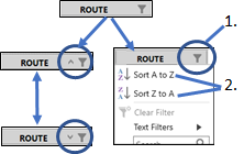
Sorting the columns in a worksheet can be accomplished by simply clicking on the column header cell. Clicking the header multiple times will toggle between ascending and descending order. A sort direction indicator is shown in the header.
Alternatively:
Click in the header.
In the popup, select Sort A to Z or Sort Z to A.
Filtering a worksheet is done through the filter icon in the column header.
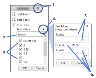
In the header of the column to be filtered, click ![]() .
.
The popup lists all values found in that column.
To search for values, begin typing the text in the Search field and the list in the popup will automatically be filtered as you type.
Use the check boxes in the list to control which rows are shown (checked boxes) or hidden (unchecked boxes) in the result worksheet. Use the (Select All) check box to check or uncheck all items in the list at the same time.
To define a filter criterion, click the Right Arrow button next to Text Filters (or Number Filters, if the column is numeric).
Use the dropdown menus to set the operators and value to set the criteria.
To include a second criteria, select the And or Or radio button and use the second set of dropdown menus to define the second criteria.