Three category multinomial model with a covariate
For this example, a completed project will be used as an illustration.
This example shows a three-category multinomial model with a covariate, run with three different engines: QRPEM, Laplacian, and Adaptive Gaussian Quadrature (AGQ). This project illustrates how to construct such a model with a simple LL statement. It also demonstrates that the results obtained by accurate methods (QRPEM and AGQ) are similar and close to the ones that are used to create the data set, while the results obtained by the approximate method (Laplacian) are relatively poor and are quite different.
Information about the example data
Select File > Load Project to open an existing Phoenix project.
In the Load Project dialog, navigate to …\Examples\NLME.
Select Multinomial_3cat_with_covariates.phxproj and press Open.
The data set consists of simulated data from a multinomial categorical model, where the observations are either y=0,1, or 2 and represent a category. The probability of an observation being a particular category is a function of four structural parameters th1, th2, th4, and th5 as follows:
Prob(y=0)=ilogit(th1+th4*PER+th5*DOSE)
Prob(y=1)=ilogit(th1+th4*PER+th5*DOSE+th2) – Prob(category=0)
Prob(y= 2)=1 – (Prob(y=1)+Prob(y=0))
Here ilogit(x)=exp(x)/(1+exp(x)) is an increasing function of its argument.
The covariate PER (period) can take the value zero or one and can vary within an individual on different occasions. Similarly, the covariate DOSE ranges from zero to 30 and can vary within an individual.
The four structural parameters have the form th1=tvth1+nh1, th2=tvth2, th4=tvth4, and th5=tvth5, where nh1 is a N(0,20) random effect associated with th1 and the nominal values of the fixed effects are: tvth1=10, tvth2=1.5, tvth4= –5, tvth5= –0.01. (These nominal values, along with the N(0,20) distribution for nh1, were used to simulate the data).
Project workflows and objects
The techniques for constructing such a multinomial model are discussed previously in the “Logistic regression modeling in Phoenix” example.
Here, the focus is on the different results from three types of methods depending on whether the method uses a low or high accuracy likelihood approximation.
There are three workflows in the model, as well as a Model Comparison object. The workflows correspond to running the same model with the QRPEM engine, a Laplacian engine, and an adaptive Gaussian quadrature engine with 21 integration points along the one-dimension random effect nh1 axis.
The QRPEM method uses 300 quasi-random sample points for its evaluation of the Bayesian posterior integrals, and thus can be considered a high accuracy method.
The Laplacian engine uses only one integration point and is often a low accuracy method, particularly in cases where the observations are categorical or counts.
The Adaptive Gaussian Quadrature engine with 21 points placed at particularly informative points is also a high accuracy method.
Note that Laplacian can be considered a special case of AGQ where only one integration point is used. In fact, the only difference between the Laplacian and AGQ21 workflows is that in the N AGQ box in the Run Options tab, the value is set to 21 for AGQ21 and to 1 for Laplacian.
Results
The results are summarized in the table below (all values are rounded to the nearest hundredth):
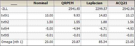
These three engines use different methods to approximate -2LL. So -2LL values cannot be used to determine which engine is better than the others. From the table above, we can see that QRPEM and AGQ21 get very good (close to nominal) estimates for all fixed effects, while the Laplacian estimates are less accurate except Tvth5. Finally, the single random effect parameter Omega is estimated very well (close to the nominal value of 20) by QRPEM and AGQ21, whereas the Laplacian estimate is very poor.