Mathematical Difference of Methods
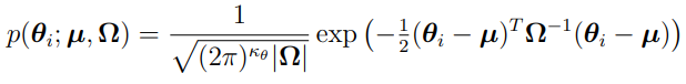
Mathematically, the difference between parametric and nonparametric method is the probability density function (PDF) of the parameters. For the parametric method, the PDF is a Gaussian, such as
(discussed in “Review of Laplacian-Approximation Formulation”)
and
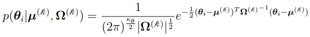
(discussed in “Two-Stage Nonlinear Random Effects Mixture Model”)
For nonparametric methods, the PDF is simply the sum of Dirac delta functions (discussed below).
Exploring the formulas
The population analysis problem can be stated as follows:
Let
 be a sequence of independent but not necessarily identically distributed random vectors constructed from one or more observations from each of NSUB subjects in the population. The {
 } are observed.
 be a sequence of independent and identically distributed random vectors belonging to a compact subset
  of Euclidean space with common but unknown distribution f. The {
 } are not observed.
Assume that the conditional densities 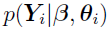 are known, for i = 1,..., n, where
  is an unknown vector in set B.
Then, the probability of given and f, can be stated as 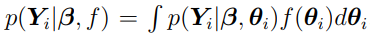 .
.
Because of the independence of {}, the probability of {}, given and f, is given by the likelihood
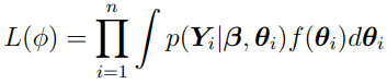
where 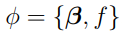 . In the context of “mixed-effects” problems, the vector describes the fixed effects and {} describes the random effects.
Thus, the population analysis problem is to maximize the likelihood function  with respect to all parameters in B and all density functions f on .
The maximum likelihood problem, as stated above, is infinite dimensional. The theorems of Mallet [6] and Lindsay [5] reduce this problem to finite dimensions. It was proved under simple hypotheses on the conditional densities , that for fixed , the optimal density f could be found in the space of discrete densities with no more than NSUB support points, where n is the number of subjects. This means K is a bounded value, making all the numerical computations feasible. Therefore, f can be written as a weighted sum of delta functions.
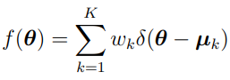
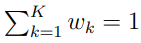
where
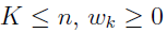 .
.
 .
.
The weights and the vector  (also known as a support point [4]) are implicit functions of .
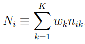
The likelihood equation now becomes
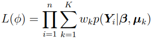
where  .
.
The quantity 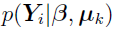 can be taken as the (i, k) element of the NSUB by the K likelihood matrix:
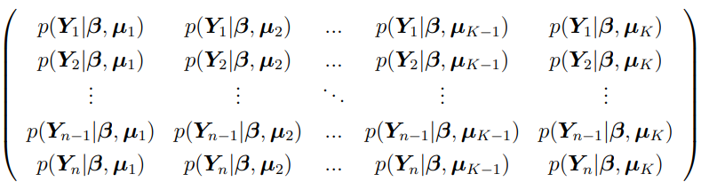
Typically, the log likelihood function for L(ϕ) is calculated as:
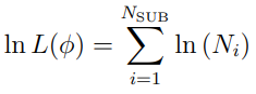
nik is the (i, k) element of the NSUB by K likelihood matrix,  .
.
In most cases, the -dimensional observation vector for the ith individual  is sampled from a Gaussian distribution such as
  (discussed in “Two-Stage Nonlinear Random Effects Mixture Model”). Thus, is simply the corresponding Gaussian.
The maximum likelihood approaches for parametric and nonparametric methods are the same. It is only due to the PDF of nonparametric approaches being the sum of delta functions, such as
instead of Gaussian that the corresponding log-likelihood function, such as
does not involve any integrals. Therefore, the calculation of log-likelihood is much faster than that in parametric methods. However, the time-consuming part for nonparametric methods, is to search for the , , the support points , and the optimum number of support points K. Note that there is no covariance matrix OMEGA in nonparametric methods.