Ordinary Differential Equations (ODEs) Solvers
Ordinary differential equations (ODEs) can be solved for Phoenix models by several methods. These methods are available under the option Max ODE in the Run Options tab.
Some models use ODE systems expressed by 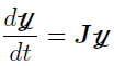 , where
 is a time-dependent column vector
 is a (Jacobian) matrix with no time-dependent elements, but may contain the infusion rate information, etc.
For such ODEs, there is no need to use numerical ODE solvers that contain time-step errors (e.g., DVERK, LSODA, LSODE, DOPRI5) as there is a simple solution of 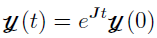 , where (0) is the initial value of at t = 0 and is known.
To get the solution  , it is important to calculate
  , which is a matrix. The two matrix exponential ODE solvers, Matrix Exponent and Exponent Higham, are used to calculate , and can only be used to calculate ODEs where the solution is . These two solvers do not need to repeatedly evaluate the ODEs and, therefore, are faster than the other numerical ODE solvers available in Phoenix. Furthermore, they are not influenced by the stiffness of the ODEs. Both Matrix Exponent and Exponent Higham use a general method called “scaling and squaring”[1] to calculate . It uses the property:
= 
where
s is the scaling parameter and a non-negative integer
 is estimated by Padé approximation
The  inside () is “scaling”
  , and the superscript
  on is “squaring” ().
Matrix exponential ODE solvers
Numerical ODE solvers
A correctly rounded mathematical library[2] is used for some elementary functions implementation to reduce the differences in results between platforms, CPUs, and operating systems.
The ODE solvers used by Phoenix have three accuracy controls that are available in the Advanced options section of the Run Options tab:
ODE Rel. Tol.: Relative tolerance (RTOL)
ODE Abs. Tol.: Absolute tolerance (ATOL)
ODE max step: Maximum number of allowable steps or function evaluations (depending on the solver) to achieve the above accuracies (MAXSTEP)
For more information, see the “RTOL, ATOL, and MAXSTEP ODE error controls” section.
This is the default option for solving ordinary differential equations for Phoenix models and is based on the DGPADM subroutine in the Expokit package developed by Roger B. Sidje [3]. As its name implies, the Matrix Exponent option uses the matrix exponential for solving ODEs. Hence, it requires that the system can be expressible as , where is a matrix (the Jacobian) with elements that are constant over a time interval. It uses “scaling and squaring” method combined with Padè approximation to calculate . It is faster and more accurate than the numerical ODE solvers and does not suffer from stiffness of the ODEs. Additional information on using the matrix exponential for solving ODEs is available in the “Matrix Exponent” section in the PML Reference Guide.
For the case where the Matrix Exponent option cannot be used for the given model, Phoenix automatically switches the ODE solver to the non-stiff solver DVERK except in the case where the model involves gammaDelay function (for this case, it automatically switches to the non-stiff solver DOPRI5). Note that the actual ODE solver requested/used can be found at the beginning of the Core Output tab (Text Output Results section).
Note: The Matrix Exponent option has a weakness manifested in a subtle phenomenon known as overscaling, which can significantly harm the accuracy of the results. For example, for the cases where the infusion rate is larger than 2^28 ~ 2E8 and the other elements in the Jacobian matrix J are relatively low (more than 8 orders of magnitudes less), it may give inaccurate results. When an overscaling is suspected, a warning message is outputted to either Core Status text output or Warnings and Errors text output or both. In such cases, it is recommended to switch to either the exponent Higham solver or the numerical ODE solvers, such as the non-stiff DVERK.
The exponent Higham option uses the matrix exponential for solving ODE but is based on a different algorithm to compute the matrix exponential. [4]
It uses the “scaling and squaring” method combined with Padè approximation to calculate . This algorithm alleviates the overscaling problem and, hence, may be more accurate than the Matrix Exponent option for certain models (e.g., models where the infusion rate is more than eight orders of magnitudes larger than the other elements in the Jacobian matrix).
LSODE (Livermore Solver for Ordinary Differential Equations)[5] is the ODE solver used by Phoenix to solve stiff systems of the form dy/dt=f. It treats the Jacobian matrix df/dy as either a dense (full) or a banded matrix, and as either supplied automatically by Phoenix or internally approximated by difference quotients (if Phoenix fails to generate it).
Stiff systems typically arise from models with processes that proceed at different rates, for example, slow equilibration of a peripheral compartment with a central compartment relative to the rate at which elimination occurs from the central compartment. Generally, a stiff solver outperforms, in terms of both time and accuracy, a non-stiff solver for such systems but the non-stiff solver can be superior for non-stiff systems.
Nonlinear systems can change from stiff to non-stiff during evaluation, which can result in incorrect estimates and/or much longer execution times if the incorrect ODE solver is selected. LSODA [5] is a variant version of the LSODE solver and it automatically selects between non-stiff and stiff methods. It uses Adams methods (predictor corrector) in the non-stiff case, and Backward Differentiation Formula (BDF) methods (the Gear methods) in the stiff case. LSODA is a robust adaptive stepwise solver that uses the non-stiff method initially, and dynamically monitors data to decide which method to use.
Based on the DVERK solver[6], this is an explicit Runge-Kutta method founded on Verner’s fifth and sixth order pair of formulas. Due to its fast and robust performance, it is one of the widely used methods for solving non-stiff problems and is also the default solver used by Phoenix when the matrix exponent solver is not applicable.
It is well-known that the explicit Runge-Kutta methods cannot compete with specifically designed stiff methods, except for very mildly stiff systems. For the stiff problems, integration errors are expected. Switch to the LSODE/LSODA solver.
DOPRI5 is another widely used solver for non-stiff problems. Based on the DOPRI5 ODE solver by E. Hairer and G. Wanner[7], it is an explicit Runge-Kutta method of order (4)5, based on Dormand-Prince pair. More specifically, it uses six function evaluations to calculate fourth- and fifth-order accurate solutions. Numerical experiments show that DOPRI5 may be more reliable and efficient than DVERK, in certain stiff problems.