Modeling circadian rhythm example
This example is based on the study of the pharmacokinetics of midazolam reported by Van Rongen, A., et al., CPT: Pharmacometrics & System Pharmacology, 4.8:454–464 (1985). The aim of this study was to evaluate 24-hour variation in the pharmacokinetics of the CYP3A substrate midazolam.
This example shows an implementation of the cosinor procedure for describing 24 hour variation. This project also illustrates the visual predictive check results with stratification on inter-occasion variables and how to implement a two dose point model with two epsilons, one for oral and the other one for IV using Textual Mode.
Open the project
Load the Phoenix project …\Examples\NLME\Midazolam_Circadian_IOV_TwoEpsilon_Estimation_VPC.phxproj.
Two datasets are listed in the Data folder. The dataset midazolam_sim consists of observations CObs, covariate OCC, which depends on the time of dosing and includes 6 dosing occasions (OCC=1 (10:00 AM) 2 (02:00 PM), 3 (06:00 PM), 4 (10:00 PM), 5 (02:00 AM), 6 (06:00 AM)), covariate OCCTime, representing the time of dosing in minutes starting at midnight, where TAD is time after dosing in minutes and is mapped to Time to avoid unnecessary computations. There are 12 subjects for each dosing period.
The input doses in the dataset midazolam_dose are the same as in the mentioned article. The PO dose separated in time from IV bolus by 150 minutes.
Review the model text
In the Object Browser, expand the Workflow and select the MidazolamModel object.
Select Model in the Setup list. The Model text panel is displayed.
The value of bioavailability (F1) oscillates around mesor, and is defined as follows:

with baseF1 defined in the stparam statement as:

Here:
tvF1 presents the typical value of bioavailability
nF1 is the inter-individual variability (eta)
IOV is the inter-occasion variability implemented in the following statement with inter-individual variability incorporated inside.
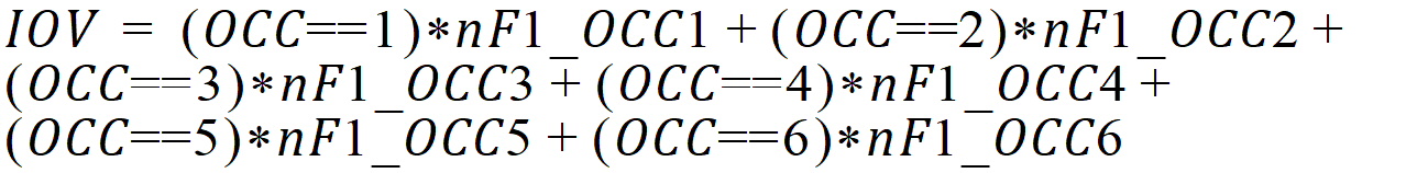
AMP is the amplitude of cosine function
FR is the period of cosine function (24 hours)
AC is the acrophase (time to peak of the cosine function)
t+OCCTime represents the time in minutes starting at midnight.
The clearance is defined similarly as the bioavailability. For the absorption rate constant Ka, a multiplication factor at 2:00 PM is added by applying of the ternary operator:

It is worth noting that the multiplication factor in the absorption rate was found in Van Rongen, A., et al. (2015) to give a better fit to the clinical data.
Note that for this example the value of the standard deviation for the residual error changes after TAD reaches 150 minutes; that is, there are two epsilons (epsilon 1: oral, epsilon 2: IV bolus 150 minutes after oral). To incorporate this, a fixed effect is introduced using the following statements:
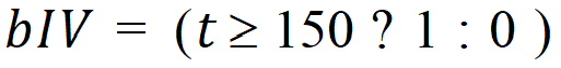


The above statements means that if TAD is less than 150 minutes, the standard deviation for the residual error is 0.163723. Otherwise, it is (1+Coeff_IV)* 0.163723.
Execution of VPC model
In the Object Browser select VPC MidazolamModel object.
This model is a copy of the previous one with the values for the fixed and random effects chosen as the final estimated parameter values.
Select the Run Options tab.
Make sure that Predictive Check run mode is selected.
In the Main sub-tab, leave the categorical covariate OCC selected from the Stratify menu.
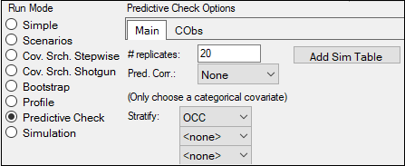
Switch to the CObs sub-tab and make sure that the Quantile box is checked.
Click ![]() (Execute icon).
(Execute icon).
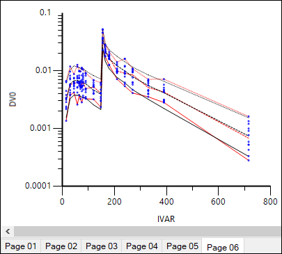
Select Pop PredCheck ObsQ_SimQ in the Plots part of the Results tab.
For each stratum, the observed quantiles are superimposed with predictive check quantiles over the observed data. The results are shown in the image below, which shows a reasonable match between observed and predicted data. Red lines: observed quantiles, black lines: predicted quantiles, blue symbols: observed data.
Select Pop PredCheck_ObsQ_SimQCI in the Plots part of the Results tab.
PredCheck_ObsQ_SimQCI plot of confidence intervals of the simulated quantiles is generated due to the checked Quantile box in the Predictive Check Options area:
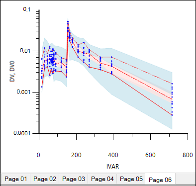
In each plot, the two blue shaded areas respectively represent the confidence intervals for the simulated 5th and 95th quantiles, and the red shaded area represents the confidence interval for the 50th quantile. The red lines inside these shaded areas denote the median of these simulated quantiles.
In this project, the lines that define the outer edge of the shaded areas have been removed by double-clicking on the plot and setting Line Style to None for each of the Predicted Quantiles graphs that named “05%, 05%” through “95%. 95%”.