Substitute estimable for non-estimable functions
It is not always easy to determine if a linear combination is estimable or not. LinMix tries to be helpful and, if a non-estimable function is encountered, will substitute a “nearby” function that is estimable. Notice is given in the text output when the substitution is made, and results should be reviewed to check the coefficients to see if they are reasonable. This section is to describe how the substitution is made.
The most common attempt to estimate a non-estimable function of the parameters is probably trying to estimate a contrast of main effects in a model with interaction, so this will be used as an example. Consider the model:
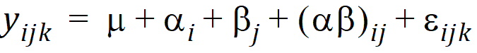
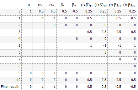
where m is the over-all mean; ai is the effect of the i-th level of a factor A,i=1, 2; j is the effect of the j-th level of a factor B, j=1, 2; (ab)ij is the effect of the interaction of the i-th level of A with the j-th level of B; and the eijk are independently distributed N(0, s2). The canonical form of the QR factorization of X is displayed in rows zero through eight of the table below. The coefficients to generate a1 – a2 are shown in row 9. The process is a sequence of regressions followed by residual computations. In the m column, row 9 is already zero so no operation is done. Within the a columns, regress row 9 on row 3. (Row 4 is all zeros and is ignored.) The regression coefficient is one. Now calculate residuals: (row 9) – 1´ (row 3). This operation goes across the entire matrix, i.e., not just the a columns. The result is shown in row 10, and the next operation applies to row 10. The numbers in the b columns of row 10 are zero, so skip to the ab columns. Within the ab columns, regress row 10 on row 5. (Rows 6 through 8 are all zeros and are ignored.). The regression coefficient is zero, so there is no need to compute residuals. At this point, row 10 is a deviation of row 9 from an estimable function. Subtract the deviation (row 10) from the original (row 9) to get the estimable function displayed in the last row. The result is the expected value of the difference between the marginal A means.
This section provides a general description of the process just demonstrated on a specific model and linear combination of elements of b. Partition the QR factorization of X vertically and horizontally corresponding to the terms in X. Put the coefficients of a linear combination in a work row. For each vertical partition, from left to right, do the following:
Regress (i.e., do a least squares fit) the work row on the rows in the diagonal block of the QR factorization.
Calculate the residuals from this fit across the entire matrix. Overwrite the work row with these residuals.
Subtract the final values in the work row from the original coefficients to obtain coefficients of an estimable linear combination.
The table below shows the QR factorization of Z scaled to canonical form.