Satterthwaite approximation for degrees of freedom
The linear model used in linear mixed effects modeling is: Y ~ N(Xb,V)
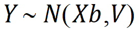
where X is a matrix of fixed known constants, b is an unknown vector of constants, and V is the variance matrix dependent on other unknown parameters. Wald (1943) developed a method for testing hypotheses in a rather general class of models. To test the hypothesis H0: Lb=0, the Wald statistic is:
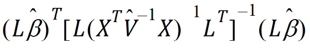
where:
 is the estimator of b.
 is the estimator of V.
L must be a matrix such that each row is in the row space of X.
The Wald statistic is asymptotically distributed under the null hypothesis as a chi-squared random variable with q=rank(L) degrees of freedom. In common variance component models with balanced data, the Wald statistic has an exact F-distribution. Using the chi-squared approximation results in a test procedure that is too liberal. LinMix uses a method based on analysis techniques described by Allen and Cady (1982) for finding an F distribution to approximate the distribution of the Wald statistic.
Giesbrecht and Burns (1985) suggested a procedure to determine denominator degrees of freedom when there is one numerator degree of freedom. Their methodology applies to variance component models with unbalanced data. Allen derived an extension of their technique to the general mixed model.
A one degree of freedom (df) test is synonymous with L having one row in the previous equation. When L has a single row, the Wald statistic can be re-expressed as:
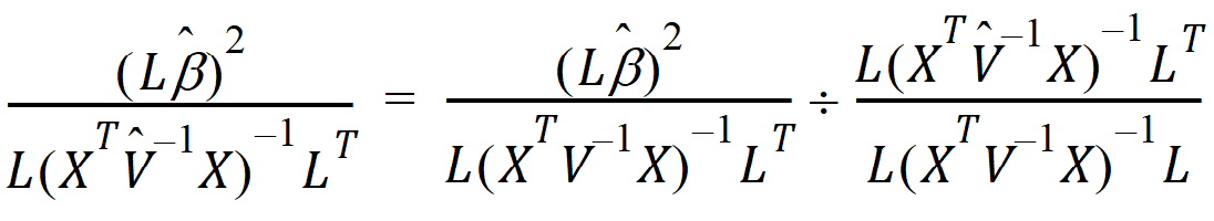
Consider the right side of this equation. The distribution of the numerator is approximated by a chi-squared random variable with 1 df. The objective is to find n such that the denominator is approximately distributed as a chi-squared variable with n df. If:
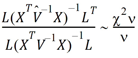
is true, then:
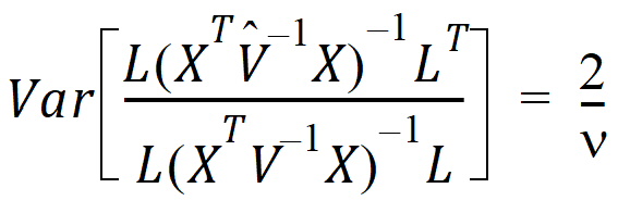
The approach is to use this equation to solve for n.
Find an orthogonal matrix R and a diagonal matrix L such that:
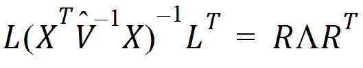
The Wald statistic equation can be re-expressed as:
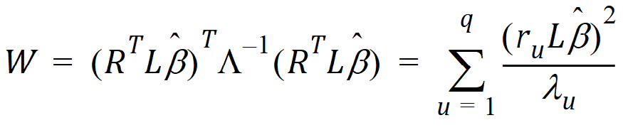
where ru is the u-th column of R, and lu is the u-th diagonal of L.
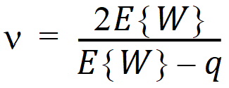
Each term in the previous equation is similar in form to the Wald statistic equation for a single row. Assuming that the u-th term is distributed F(1, nu), the expected value of W is:
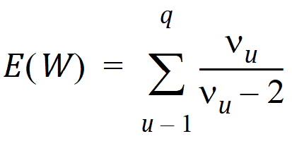
Assuming W is distributed F(q, n), its expected value is qn/(n – 2). Equating expected values and solving for n, one obtains: