The_delay_function

The delay function

The delay function in PML can be used for both discrete delay and distributed delay (gamma, Weibull, and inverse Gaussian distribution are supported) and its syntax is given as follows:

    delay(S, MeanDelayTime 
         [, shape = ShapeParam] 
         [, hist = HistExpression]
         [, dist = NameOfDistribution]
         )

If the shape option is not provided, then it describes a discrete delay and returns the value of:

S(t − MeanDelayTime)

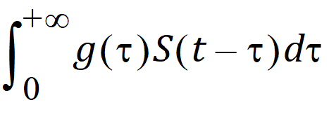
Otherwise, it describes a distributed delay and returns the value of:

Phoenix_UserDocs_PML_image1571

Here, g denotes the probability density function of the distribution specified in the dist option (whose value can be Gamma, Weibull, or InverseGaussian) with its shape parameter speciﬁed by the shape option and mean being MeanDelayTime. The hist option is used to specify the value of S prior to time 0; that is, if t < 0, then S(t)=HistExpression, which is required to be independent of time t but can depend on variables that are defined at time 0 for the subject, such as covariates, ﬁxed and random eﬀects. If the hist option is not provided, then it is assumed that S(t)=0 for t < 0. If the dist option is not provided, then dist=Gamma is assumed.

It should be noted that the delay function relies on the fact that ODE solvers use shorter step sizes in the vicinity of rapid changes. Hence, it will not work in the presence of methods that have large step sizes, such as matrix exponent or closed-form. Even though there is no restriction on the number of delay functions put in a model, it should be used sparingly to avoid performance issues.

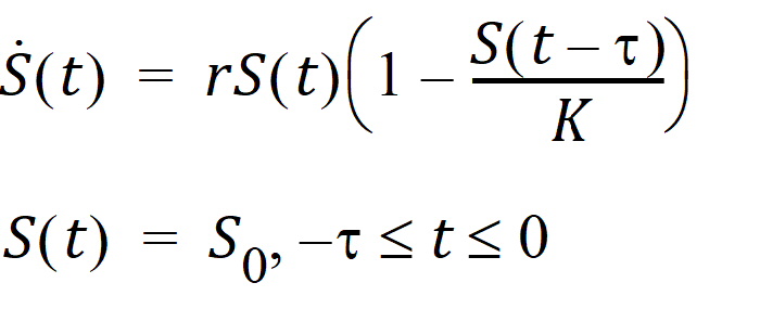
For the discrete delay function, the delay time can be estimated, and for the distributed delay case, both the mean and shape parameter for the specified distribution can be estimated. In addition, the delay function can be put on the right-hand side of a differential equation, and hence can be used to numerically solve a differential equation with either discrete delays or distributed delays, no matter whether the signal to be delayed, S, depends on model states or not. For example, the delay function can be used to numerically solve the well-known Hutchinson equation (a logistic growth model with a discrete delay):

Phoenix_UserDocs_PML_image1573

where r denotes the intrinsic growth rate, K is the carrying capacity, and S₀ is a positive constant. The PML code for this model is given as follows:

    deriv(S=r*S*(1-delay(S, tau, hist=S0)/K)) 
    sequence{S=S0}

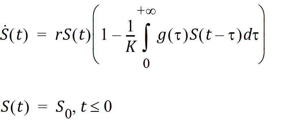
The delay function can also be used to numerically solve the following logistic growth model with a distributed delay:

Phoenix_UserDocs_PML_image1575

where g is the probability distribution function of the supported distribution (gamma, Weibull, or inverse Gaussian) with shape parameter being ShapeParam and mean being MeanDelayTime. The PML code for this model with a Weibull distributed delay is given as follows:

    delayedS = delay(S, MeanDelayTime, 
         shape = ShapeParam, 
         hist = S0, 
         dist = Weibull
         ) 
    deriv(S = r*S*(1-delayedS/K)) 
    sequence{S = S0}

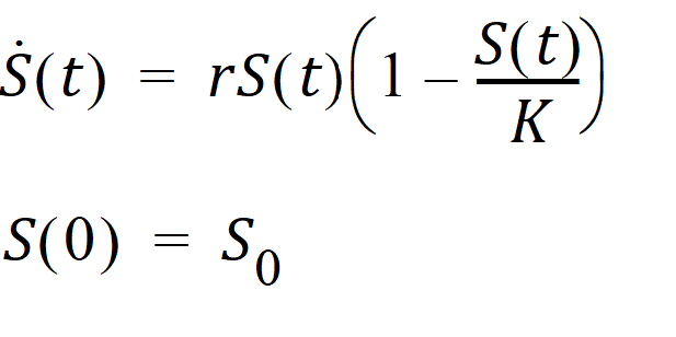
A simple simulation of the logistic growth model with a gamma distributed delay (the previous equation) is given in example project LogisticGrowthModelWithGammaDistributedDelay.phxproj (located in …\Examples\NLME). The project demonstrates that the previous equation can exhibit much richer dynamics than its corresponding ODE.

Phoenix_UserDocs_PML_image1577

For example, it may produce an oscillation around the carrying capacity while the corresponding ODE cannot. In addition, adjusting the mean delay time can achieve the desired type of oscillations (either damped or sustained oscillations).