Note that, the signal to be delayed, S, in the delay function cannot contain dosing information from the input data set. Hence, it cannot be used for the absorption delay case. To achieve this, a compartment modeling statement, delayInfCpt, was added to PML with its syntax given as follows:
    delayInfCpt(A, MeanDelayTime,
         ParamRelatedToShape
         [, in = inflow]
         [, out = outflow]
         [, dist = NameOfDistribution]
         )
Here, A denotes a compartment that can receive doses (from the input data set) through the dosepoint statement. The second and third arguments are used to characterize the distribution specified in the dist option, which has values of Gamma, Weibull, and InverseGaussian. Specifically, the second argument denotes the mean of the specified distribution, and the third argument is related to the shape parameter of the specified distribution:
If dist = InverseGaussian, then ParamRelatedToShape = ShapeParameter,
Otherwise, ParamRelatedToShape is set to be ParamRelatedToShape = ShapeParameter–1, and it must be non-negative to prevent the shape parameter from being less than one (which causes a singularity of the probability density function of the gamma or Weibull distribution at time 0).
The optional in option is used to specify any additional flow that is delayed with its history function assumed to be zero. The optional out option is used to specify flow rates (either out of or into compartment A) that are not delayed. If the dist option is not provided, then the system automatically assumes that dist = Gamma.
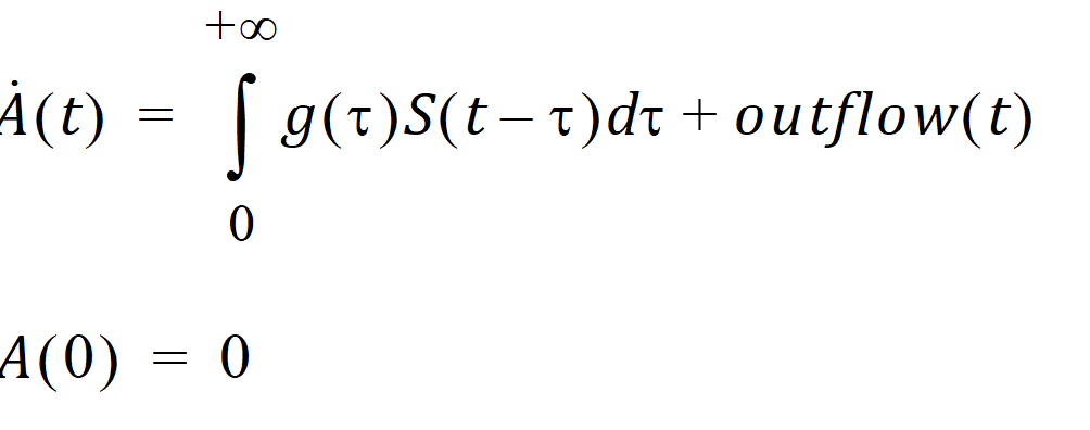
Mathematically, the delayInfCpt statement means:

Here S denotes all the input to be delayed, including the dose and the inflow specified by the in option, with S(t)=0 if t < 0, and g is the probability distribution function of the distribution specified by the dist option. The outflow is defined by the out option.
There are two examples that demonstrate how to use delayInfCpt to model absorption delay. For the first one, the delay time between the administration time of the drug and the time when the drug molecules reach the central compartment is assumed to be gamma distributed with the mean given by MeanDelayTime and shape parameter ν given by ν=ShapeParamMinusOne+1. In addition, the drug is assumed to be described by a one-compartment model with a first-order clearance rate. The PML code for the structure model of this example is then given by:
    # central compartment
    delayInfCpt(A1, MeanDelayTime,
         ShapeParamMinusOne,
         out =-Cl*C
         )
    dosepoint(A1)
    # drug concentration at the central compartment
    C=A1/V
The second example is about double sites of absorption, where the drug is assumed to be described by a two-compartment model with a first-order elimination from the central compartment. In addition, the delay time between the administration time of the drug and the time when the drug molecules reach the central compartment is assumed to be gamma distributed for each pathway. The PML code for the structure model of this example is then given by:
    # 1st pathway contribution to the central compartment,
    # where frac denotes the fraction of dose absorbed by
    # the 1st pathway, and the remaining dose is
    # absorbed by the 2nd pathway.
    (Ac1, MeanDelayTime1, ShapeParamMinusOne1,
         out=-Cl*C-Cl2*(C-C2)
         )
    dosepoint(Ac1, bioavail=frac)
    # 2nd pathway contribution to the central compartment
    delayInfCpt(Ac2, MeanDelayTime2, ShapeParamMinusOne2)
    dosepoint(Ac2, bioavail=1-frac)
    # Peripheral compartment
    deriv(A2=Cl2*(C-C2))
    # Drug concentration at the central compartment
    C=(Ac1+Ac2)/V
    # Drug concentration at the peripheral compartment
    C2=A2/V2
The model fitting for the first example (called gamma absorption delay model) is demonstrated in the example project ModelAbsorptionDelay_delayInfCpt.phxproj (located in …\Examples\NLME). In the project, there are two other models that are the same as the gamma absorption delay model but with the absorption delay time assumed to be either inverse Gaussian distributed (called inverse Gaussian absorption delay model) or Weibull distributed (called Weibull absorption delay model). The estimation results obtained for these three models show that the shape parameter and the mean delay time can be reliably estimated along with the other parameters. In addition, standard diagnostic plots are good.
The Model Comparer tool is then used to compare these three models and shows that the gamma absorption delay model is the best one to describe the given data (in terms of having a lower AIC/BIC value), see the workflow ModelComparer in the project for details. The visual predictive check (VPC) is then performed for the gamma absorption delay model with initial estimates for Theta, sigma, and Omega set to their corresponding final estimates (by using the Accept All Fixed+Random button in the Parameters > Fixed Effects sub-tab to accept the final parameter estimates as the initial estimates), see the workflow VPC in the project for details. The VPC plots suggest that the gamma absorption delay model provides a good explanation of the data.