Multi statement for Categorical models
    multi(observedVariable, inversLinkFunction(, expression)*
       [, actionCode])
This statement specifies an integer-valued categorical observed variable. The name of an inverseLinkFunction is given, and it can be ilogit, iprobit, iloglog. The next part of the statement is a series of expressions in ascending order, such as C-X01 or C-X12, where X01 is the value of C that evenly divides the response between zero and one, and X12 divides the response between one and two. These expressions are the inputs to the inverse link function
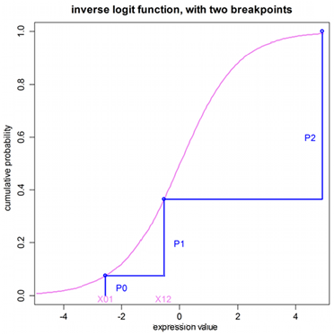
This relationship between offset expressions is illustrated below but without using a variable in the expression. The domain of the parameters X01 and X12 exists along the unbounded real line. The goal is to divide the range of the inverse function (0,1) into the probabilities of the categorical observations. This preserves the constraint that the sum of the probabilities equals one.
In the illustration below, the first breakpoint, proceeding from left to right, is X01. The value of the inverse function (ilogit, in this case) is taken at X01 and P0, which is the probability of the first category, is P0=ilogit(X01). The next breakpoint is X12, and the probability of observing the second category is P1=ilogit(X12)-ilogit(X01), which is the cumulative probability between the first and second breakpoints. The third observation has probability P2=1-P0-P1, which is the remainder of the cumulative probability.

It is simple to extend the example beyond simple values of X01 and X12, to include a function of covariates. Given the relationship between the category probabilities and the probabilities, it is easy to see why the initial estimates of the parameters should be given in such a way as to not cause the computed values of any of the probabilities to be negative. It is imperative that initial conditions be chosen carefully to ensure convergence.
All about Multinomial (ordered categorical) responses
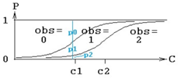
Consider a model in which an observation can take values zero, one, and two. No matter what value concentration C is, any value of the observation is possible, but C affects the relative probabilities of the observed values. If C is low, the likely observation is zero. If it is high, the likely observation is two. In the middle, there is a value of C at which an observation of one is more likely than at other values of C.
The following figure illustrates the concept. At any value of C, there is a probability of observing zero, called p0. Similarly for one and two. The probability is given by the inverse of a link function, typically logit. In this picture, there are two curves. The left-hand curve is ilogit(C-c1) and it is the probability that the observation is ³1. The right-hand curve is ilogit(C-c2), and it is the probability that the observation is ³2. The probability of observing one (p1) is the difference between the two curves. When doing model-fitting, the task is to find the optimum values c1 and c2. Note that c2 is the value of C at which the probability of observing two (p2) is exactly 1/2, and that c1 is the value of C at which the probability of observing a value greater than or equal to one (p1+p2) is exactly 1/2. Note also that c1 and c2 have to be in ascending order, resulting in the curves being in descending order.

There are statements in PML for modeling such a response: multi, and ordinal, and it can also be done with the general log-likelihood statement, LL. The multi statement for the above picture is this:
multi(obs, ilogit, C-c1, C-c2)
obs is the name of the observed variable, ilogit is the inverse link function, and the remaining two arguments are the inputs to the inverse link function for each of the two curves. Since c1 and c2 are in ascending order, the inputs for the curves, C-c1 and C-c2, are in descending order.
A more widely accepted way to express such a model is given by logistic regression, as in:
P(obs >= i)=ilogit(b*C+ai)where b is a slope (scale) parameter, and each ai is an intercept parameter. The ordinal statement expresses it this way (see the “Ordinal statement for Ordinal Responses” section):
ordinal(obs, ilogit, C, b, a1, a2)
where the ai are in ascending order. This is equivalent to the multi statement:
multi(obs, ilogit, -(b*C+a1), -(b*C+a2))
where, since the ai are in ascending order, the arguments -(b*C+ai) are in descending order, as they must be for the multi statement.
To do all this with the log-likelihood statement (LL) requires calculating the probabilities oneself, as shown below. Using the original parameterization with c1 and c2:
   pge1=ilogit(C-c1)
   pge2=ilogit(C-c2)
   LL(obs, obs==0?log(1-pge1):
           obs==1?log(pge1-pge2):
                  log(pge2)
   )
The first statement computes the first curve, the probability that the observation is greater than or equal to one, pge1. The second statement computes the second curve, the probability that the observation is greater than or equal to two, pge2. Note that these are in descending order because the probability of observing two must be less than (or equal to) the probability of observing one or two.
The third statement says obs is the observed variable, and if its value is zero, then its log-likelihood is the log of the probability of zero, where the probability of zero is one minus the probability of greater than or equal to one, i.e., log(1-pge1). Similarly, if the observation is one, its probability is pge2-pge1. Note that since pg1e>pge2, the probability of one is non-negative. Similarly, if the observation is two, its probability is pge2-pge3, where pge3 is zero because three is not a possible observation.
If, on the other hand, the typical slope-intercept parameterization from logistic regression was used, the first two lines of code would look like this:
   pge1=ilogit(-(b*C+a1))
   pge2=ilogit(-(b*C+a2))
and the LL statement would be the same.