Event statement for Time-to-event models
event(observedVariable, expression [, actionCode])
Specifies an occur observedVariable, which has two values: 1, which means the event occurred, or 0, which means the event did not occur. The hazard is given by the expression.
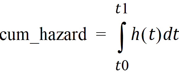
The event statement creates a special hidden differential equation to accumulate, or integrate, the hazard rate, which is defined by the expression in the second argument. This integration is reset whenever the occur variable is observed, so the integral extends from the time t0 of the previous occur observation to t1, the time of the current observation. Let cum_hazard=integral of the hazard during the period [t0,t1]:

Then the probability that an event will not occur in the period is: S=exp(-cum_hazard). Therefore, if the period terminates with an observation occur=0 at t1, the likelihood is S. If the period terminates at t1 because an event occurred at time=t1 (occur=1), then the likelihood is S*hazard(t1), where hazard(t1) is the hazard rate at t1. These likelihood computations are performed automatically whenever an occur observation is made.
Note: The observations of 0 (no event) can occur at pre-defined sampling points but observations of 1 (event occurred) are made at the time of the event.
Event models are inherently time-based and require a mapping for a time value.
All about Time-to-Event modeling
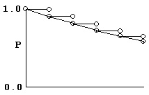
Consider a process modeled as a series of coin-tosses, where at each toss, if the coin comes up “heads,” that means an event occurred and the process stops. Otherwise, if it comes up “tails,” the coin is tossed again. The graph below shows that process if the probability of “heads” is 0.1, and the probability of “tails” is 0.9.

It is easy to see that the probability of getting to time 5 without getting a “heads” is 0.9 multiplied by itself 5 times. Similarly, the probability of getting a “heads” at time 5 is 0.1 multiplied by the probability of getting to time 4 without getting “heads” or 0.94*0.1.
To put it in symbols, if the probability of “heads” is p, then the probability of “heads” at time n is:
(1 – p)(1 – p) … n – 1 times … (1 – p) p
Since in model fitting the log of the probability is desired, and since, if p is small, log(1 – p) is basically –p, it can be said that the log of the probability of “heads” at time n is:
–p –p … n – 1 times … –p+log(p)
Note that p does not have to be a constant. It can be different at one time versus another.
The concept of “hazard,” h, is simply probability per unit time. If one cuts the time between tosses in half and cuts the probability of “heads” in half, the process has the same hazard. It also has much the same shape, except that the tossing times come twice as close together. In this way, the time between tosses can become infinitesimal and the curve becomes smooth.
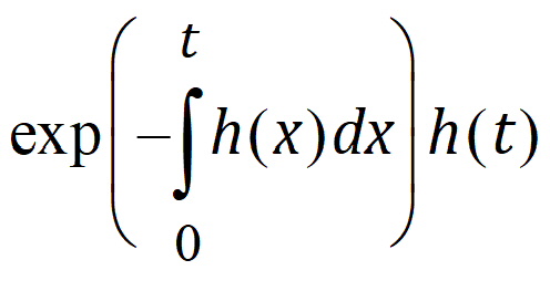
If one looks at it that way, then the probability that “heads” occurs at time t is just:

where the exponential part is the probability of no “heads” up to time t, and h(t) is the instantaneous probability of “heads” occurring at time t. Again, note that hazard h(t) need not be constant over time. If h(t) is simply h, then the above simplifies to the more familiar: exp(–ht)h.
The log of the probability is:

In other words, it consists of two parts. One part is the negative time integral of the hazard, and that represents the log of the probability that nothing happened in the interval up to time t. The second part is the log of the instantaneous hazard at time t, representing the probability that the event occurred at time t. (Actually, this last term is log(h(t) + 10-8) as a protection against the possibility that h(t) is zero.)
The event statement models this process. It is simple:
event(occur, h)
where h is an arbitrary hazard function and occur is the name of an observed variable. occur is observed on one or more lines of the input data. If its value is 1 on a line having a particular time, that means the event occurred at that time, and it did not occur any time prior, since the beginning or since the time of the prior observation of occur.
If the observed value of occur is 0, that means the event did not happen in the prior time interval, and it did not happen now. This is known as “right censoring” and is useful to represent if subjects, for example, withdraw from a study with no information about what happens to them afterward. It is easy to see how the log-likelihood of this is calculated. It is only necessary to omit the log(h) term.
Other kinds of censoring are possible. If occur equals 2, that means the event occurred one or more times in the prior interval, but it is not known when or how many times. If occur is a negative number like -3, that means the event occurred three times in the prior interval, but it is not known when. There is a special value of occur, -999999, meaning there is no information at all about the prior interval, as if the subject had amnesia. These are all variations on “interval censoring.” The log-likelihoods for all these possibilities are easily understood as variations on the formulas above.
This can be done with the log-likelihood (LL) statement instead, as follows:
   deriv(cumhaz=h)
   LL(occur, -cumhaz+occur*log(h), doafter={cumhaz=0})
The deriv statement is a differential equation that integrates the hazard. The LL statement says that variable occur is observed and it is either 1 (the event occurred) or 0 (it did not occur). It gives the log-likelihood in either case. Then, after performing the observation, the accumulated hazard is set to zero. This allows for the possibility of multiple occurrences.